CSC2626 Imitation Learning for Robotics
Week 9: Adversarial Imitation Learning
Today’s agenda
• Adversarial optimization for imitation learning (GAIL)
• Adversarial optimization with multiple inferred behaviors (InfoGAIL)
• Model based adversarial optimization (MGAIL)
• Multi-agent imitation learning
Detour: solving MDPs via linear programming
\(\underset{v}{\arg\min} \quad \underset{s \in S}{\sum} d_s v_s\)
\(\text{subject to:} \quad v_s \geq r_{s,a} + \gamma \underset{s' \in S}{\sum} T_{s,a}^{s'} v_{s'} \quad \forall s \in S, a \in A\)
\(\qquad \qquad \quad d\) is the initial state distribution.
Optimal policy
\(\pi^*(s) = \underset{a \in A}{\text{argmax}} Q^*(s, a)\)
Detour: solving MDPs via linear programming
\(\underset{\mu}{\text{argmax}} \underset{s \in S, a \in A}{\sum} \mu_{s,a} r_{s,a}\)
\(\text{subject to} \quad \underset{a \in A}{\sum} \mu_{s',a} = d_{s'} + \gamma \underset{s \in S, a \in A}{\sum} T_{s,a}^{s'} \mu_{s,a} \quad \forall s' \in S\)
\(\qquad \qquad \quad \mu_{s,a} \geq 0\)
Discounted state action counts / occupancy measure
\(\mu(s,a) = \underset{t=0}{\sum}^{\infty} \gamma^t p(s_t = s, a_t = a)\)
Optimal policy
\(\pi^*(s) = \underset{a \in A}{\text{argmax}} \, \mu(s,a)\)
Detour: solving MDPs via linear programming
\(\underset{v}{\text{argmin}} \underset{s \in S}{\sum} d_s v_s\)
\(\text{subject to} \quad v_s \geq r_{s,a} + \gamma \underset{s' \in S}{\sum} T_{s,a}^{s'} v_{s'} \quad \forall s \in S, a \in A\)
\(\qquad \qquad \quad d\) is the initial state distribution
\(\underset{\mu}{\text{argmax}} \underset{s \in S, a \in A}{\sum} \mu_{s,a} r_{s,a}\)
\(\text{subject to} \quad \underset{a \in A}{\sum} \mu_{s',a} = d_{s'} + \underset{s \in S, a \in A}{\sum} T_{s,a}^{s'} \mu_{s,a} \quad \forall s' \in S\)
\(\qquad \qquad \quad \mu_{s,a} \geq 0\)
Primal LP
Dual LP
Background
▶ Definitions: Action space \(\mathcal{A}\) and sample space \(\mathcal{S}\). \(\Pi\) is the set of all policies. Also assume \(P(s'|s,a)\) is the dynamics model. In this paper, \(\pi_E\) denotes the expert policy.
▶ Imitation Learning: Learning to perform a task from expert demonstrations without querying the expert while training.
▶ Behavioral cloning: Its success depends on large amounts of data.
▶ Inverse RL: The paper adopts the maximum causal entropy IRL which fits a cost function \(c\) with the following problem.
\[\pi^* = \arg \min_{\pi \in \Pi} -H(\pi) + \mathbb{E}_\pi[c(s,a)]\]
\[\tilde{c} = \arg \max_{c \in \mathcal{C}} \mathbb{E}_{\pi^*}[c(s,a)] - \mathbb{E}_{\pi_E}[c(s,a)]\]
where \(H(\pi) = \mathbb{E}_\pi[-\log \pi(a|s)]\) is the entropy of the policy.
Formulation
▶ We first study the policies found by RL on costs learned by IRL on the largest possible set of cost functions \(\mathcal{C} = \{c : S \times A \to \mathbb{R}\}\).
▶ Also need to define a convex cost function regularizer \(\psi : \mathbb{R}_{S \times A} \to \mathbb{R}\), which turns out to be important in this paper.
▶ Re-write the Eq. 1 as the following:
\[IRL_\psi(\pi_E) = \arg \max_{c \in \mathcal{C}} -\psi(c) + (\min_{\pi \in \Pi} -H(\pi) + \mathbb{E}_\pi[c(s,a)])\]
\[- \mathbb{E}_{\pi_E}[c(s,a)]\]
▶ Define \(RL(c) = \arg \min_{\pi \in \Pi} -H(\pi) + \mathbb{E}_\pi[c(s,a)]\).
Let \(\tilde{c} \in IRL_\psi(\pi_E)\). We are interested in characterizing the induced policy \(RL(\tilde{c})\).
Derivations
▶ It is easier to characterize \(RL(\tilde{c})\) if we transform optimization problems over policies into convex problems.
▶ So the paper introduces an occupancy measure \(\rho_\pi : S \times A \to \mathbb{R}\):
\[\rho_\pi(s,a) = \pi(a|s) \sum_{t=0}^{\infty} \gamma^t P(s_t = s|\pi) \qquad (1)\]
It can be interpreted as the distribution of state-action pairs when roll-out with policy \(\pi\).
▶ There is an one-to-one correspondence between policy and occupancy measure. It also allows us to re-write the expected cost as
\[\mathbb{E}_\pi[c(s,a)] = \sum_{s,a} \rho_\pi(s,a)c(s,a) \qquad (2)\]
Derivations
▶ Lemma 1: If we define
\[\hat{H}(\rho) = -\sum_{s,a} \rho(s,a) \log(\rho(s,a)/\sum_{a'} \rho(s,a')) \qquad (3)\]
then we have \(\hat{H}(\rho) = H(\pi_\rho)\) and \(H(\pi) = \hat{H}(\rho_\pi)\). So we can represent the entropy of a policy \(\pi\) with the occupancy measure \(\rho_\pi\).
▶ Lemma 2: If we define,
\[L(\pi, c) = -H(\pi) + \mathbb{E}_\pi[c(s,a)]\]
\[\hat{L}(\rho, c) = -\hat{H}(\rho) + \sum_{s,a} \rho(s,a)c(s,a)\]
then we have \(L(\pi, c) = \hat{L}(\rho_\pi, c)\) and \(\hat{L}(\rho, c) = L(\pi_\rho, c)\). The Lemma allows us to transform the problem from optimizing \(\pi\) to \(\rho\).
Convex Conjugate
▶ Given a function \(f\), it can be represented by the supremum of all affine functions that are majorized by \(f\).
▶ For any given slope \(m\), there may be many different constants \(b\) such that the affine function \(\langle m, x \rangle - b\) is majorized by \(f\). We only need the best such constant.
▶ That’s what the convex conjugate \(f^*\) does. Given a slope \(m\), \(f^*\) returns the best constant \(b\) such that \(\langle m, x \rangle - b\) is majorized by \(f\). Thus,
\[f^*(m) = \sup_x \langle m, x \rangle - f(x)\]
▶ Note that \(f^{**} = f\).
There is a nice visualization of convex conjugate at https://remilepriol.github.io/dualityviz/
Derivations
▶ By Lemma 2, if \(\psi\) is a constant regularizer and \(\tilde{c} \in IRL_\psi(\pi_E)\) and \(\hat{\pi} \in RL(\hat{c})\), then \(\rho_{\hat{\pi}} = \rho_{\pi_E}\).
▶ Furthermore, we can also get the main result of the paper
\[RL \circ IRL_\psi(\pi_E) = \arg \min_{\pi \in \Pi} -H(\pi) + \psi^*(\rho_\pi - \rho_{\pi_E}) \qquad (4)\]
where \(\psi^*\) is the convex conjugate of \(\psi\), which is defined as
\[\psi^*(m) = \sup_{x \in \mathbb{R}^{S \times A}} m^T x - \psi(x)\]
▶ It tells us that the \(\psi\)-regularized inverse RL seeks a policy whose occupancy measure is close to the expert’s as measured by the convex function \(\psi^*\).
▶ A good imitation learning algorithm boils down to a good choice of the regularizer \(\psi\).
Occupancy Measure Matching
▶ As we showed previously, if \(\psi\) is a constant, then the resulting policy would have the same occupancy measures with expert at all states and actions.
▶ It is not practically useful because most of the occupancy measure of the expert values are exactly zero, due to the limited expert samples.
▶ Thus, exact occupancy measure matching will force the learned policy to never visit the unseen state-action pairs.
▶ If we restrict the class of cost function \(\mathcal{C}\) to be convex and set the regularizer \(\psi\) to be the indicator function of the set \(\mathcal{C}\). Then optimization problem in (6) can be written as
\[\min_\pi -H(\pi) + \max_{c \in \mathcal{C}} \mathbb{E}_\pi[c(s,a)] - \mathbb{E}_{\pi_E}[c(s,a)] \qquad (5)\]
which is a entropy-regularized apprenticeship learning problem.
Apprenticeship Learning
▶ Policy gradient method can be used to update the parameterized policy \(\pi_\theta\) to optimize the apprenticeship objective, Eq. 7.
\[\nabla_\theta \max_{c \in \mathcal{C}} \mathbb{E}_{\pi_\theta}[c(s,a)] - \mathbb{E}_{\pi_E}[c(s,a)] = \nabla_\theta \mathbb{E}_{\pi_\theta}[c^*(s,a)]\]
\[= \mathbb{E}_{\pi_\theta}[\nabla_\theta \log \pi_\theta(a|s) Q_{c^*}(s,a)]\]
where
\[c^* = \arg \max_{c \in \mathcal{C}} \mathbb{E}_{\pi_\theta}[c(s,a)] - \mathbb{E}_{\pi_E}[c(s,a)] \qquad (6)\]
\[Q_{c^*}(\bar{s}, \bar{a}) = \mathbb{E}_{\pi_\theta}[c^*(\bar{s}, \bar{a})|s_0 = \bar{s}, a_0 = \bar{a}] \qquad (7)\]
▶ Fit \(c_i^*\) as defined above. Analytical solution is feasible if \(\mathcal{C}\) is restricted to Convex or Linear cost classes.
▶ Given the \(c_i^*\), compute the policy gradient and take a TRPO step to produce \(\pi_{\theta_{i+1}}\).
GAIL
▶ Apprenticeship learning via TRPO is tractable in large environments but is incapable of exactly matching occupancy measures without careful tuning due to the restrictive cost classes \(\mathcal{C}\).
▶ Constant regularizer \(\psi\) leads to exact matching but is intractable in large environments. Thus, GAIL is proposed to combine the best of both methods.
\[ \psi_{GA}(c) \triangleq \begin{cases} \mathbb{E}_{\pi_E}[g(c(s,a))] & \text{if } c < 0 \\ +\infty & \text{otherwise} \end{cases} \]
where
\[ g(x) = \begin{cases} -x - \log(1 - e^x) & \text{if } x < 0 \\ +\infty & \text{otherwise} \end{cases} \]
GAIL
▶ The GAIL regularizer \(\psi_{GA}\) places low penalty on cost functions \(c\) that assign an amount of negative cost to expert state-action pairs; It havily penalizes \(c\) if it assigns large cost to the expert.
▶ \(\psi_{GA}\) is an average over expert data so it can adjust to arbitrary expert datasets.
▶ In comparison, if \(\psi\) is an indicator function (Apprenticeship Learning), then it’s always fixed.
▶ Another property of \(\psi_{GA}\) is its convex conjugate \(\psi_{GA}^*(\rho_\pi - \rho_{\pi_E})\) can be derived in the following form:
\[\max_{D \in (0,1)^{S \times A}} \mathbb{E}_\pi[\log(D(s,a))] + \mathbb{E}_{\pi_E}[\log(1 - D(s,a))] \qquad (8)\]
▶ It can be interpreted to find a discriminator that distinguishes trajectory between learned policy and expert policy. t
GAIL
▶ Combining with the main result Eq. (6) in the paper,
\[RL \circ IRL_\psi(\pi_E) = \arg \min_{\pi \in \Pi} -H(\pi) + \psi^*(\rho_\pi - \rho_{\pi_E})\]
The imitation learning problem is equivalent to find a saddle point \((\pi, D)\) of the expression
\[\mathbb{E}_\pi[\log(D(s,a))] + \mathbb{E}_{\pi_E}[\log(1 - D(s,a))] - \lambda H(\pi) \qquad (9)\]
▶ In terms of implementation, we just need to fit a parameterized policy \(\pi_\theta\) with weights \(\theta\) and a discriminator network \(D_w : S \times A \to (0,1)\) with weights \(w\).
▶ Update \(D_w\) with Adam and update \(\pi_\theta\) with TRPO iteratively.
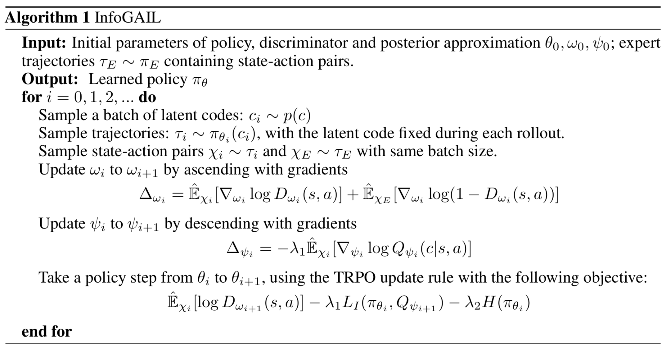
Algorithm
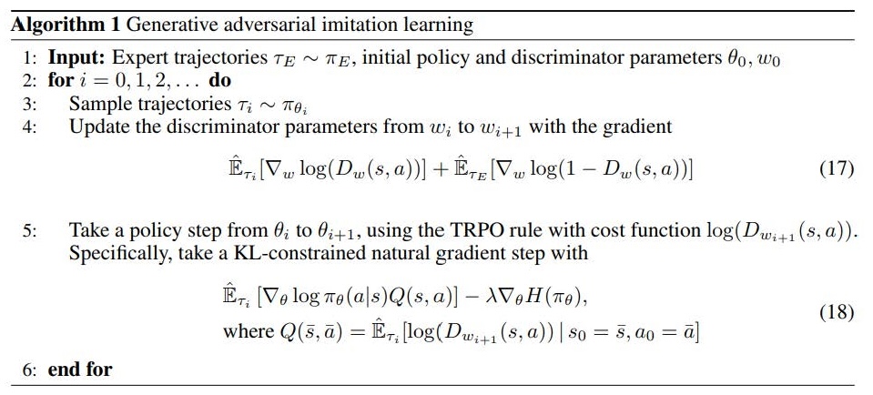
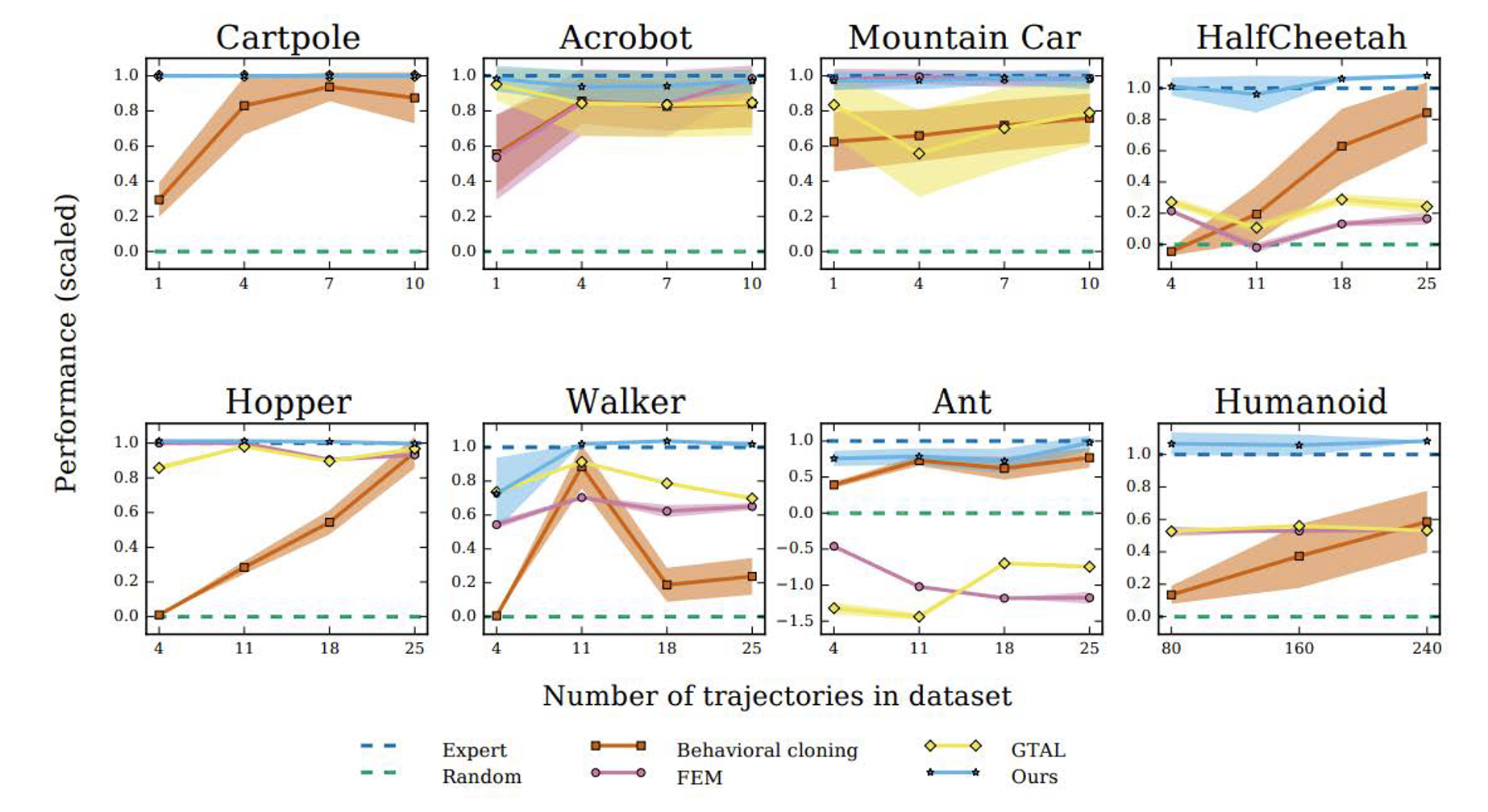
Results
Today’s agenda
• Adversarial optimization for imitation learning (GAIL)
• Adversarial optimization with multiple inferred behaviors (InfoGAIL)
• Model based adversarial optimization (MGAIL)
• Multi-agent imitation learning
InfoGAIL: Interpretable Imitation Learning from Visual Demonstrations
Presenter: Yin-Hung Chen
Motivation
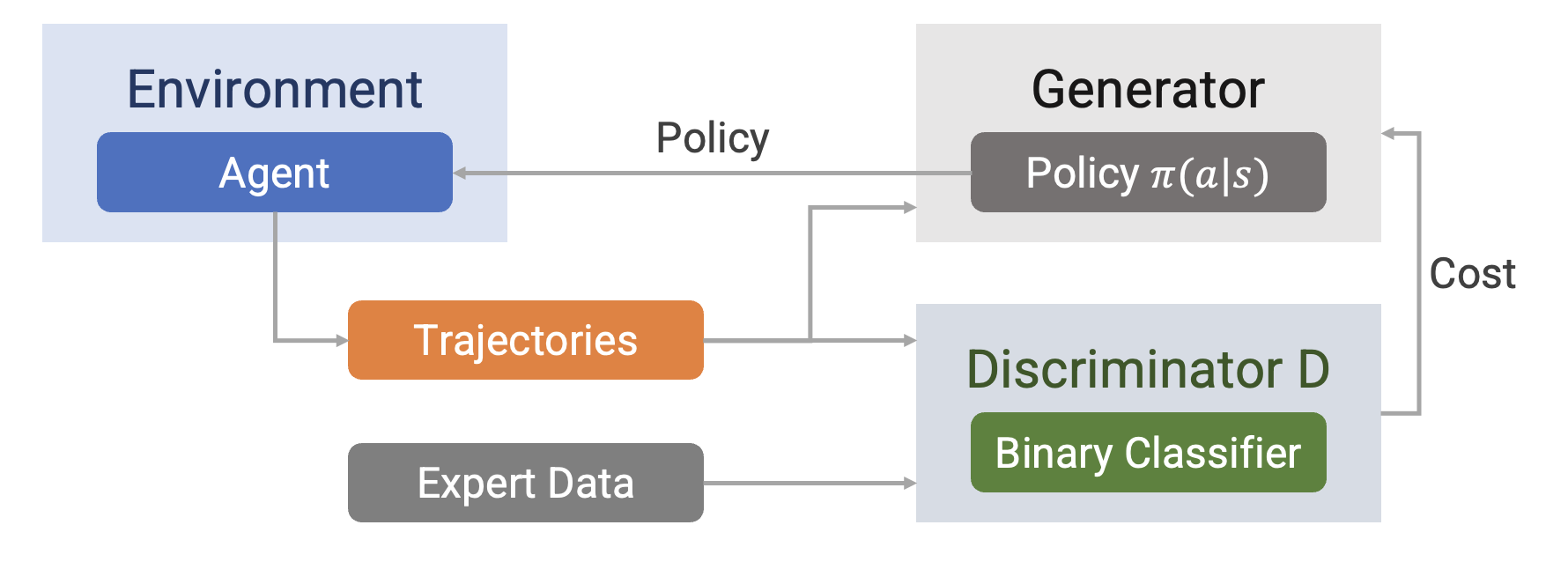
GAIL
A generator producing a policy 𝜋 competes with a discriminator distinguishing 𝜋 and the expert.
Drawbacks of GAIL
Expert demonstrations can show significant variability.
The observations might have been sampled from different experts with different skills and habits.
External latent factors of variation are not explicitly captured by GAIL, but they can significantly affect the observed behaviors.
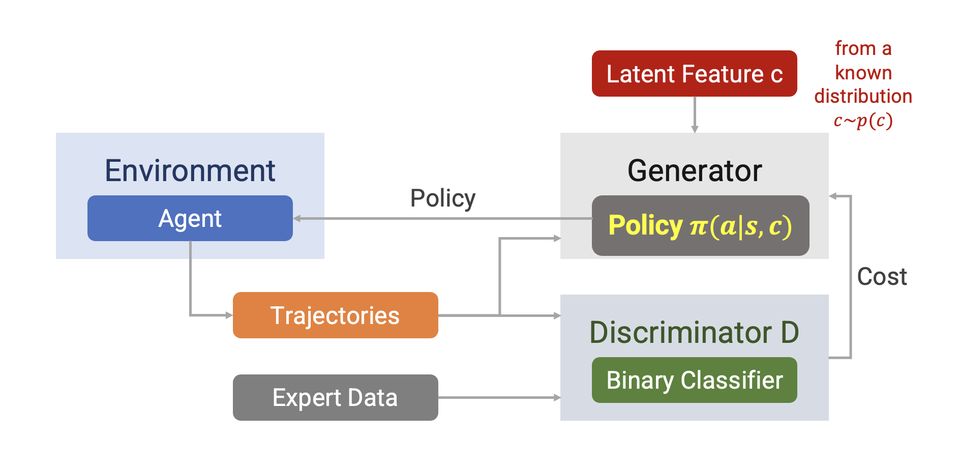
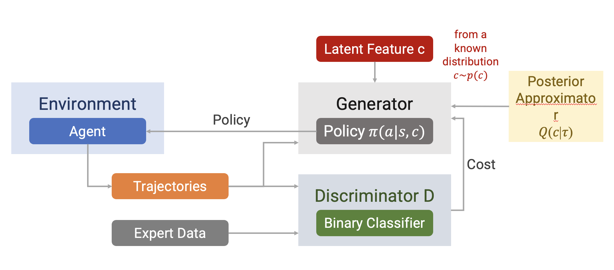
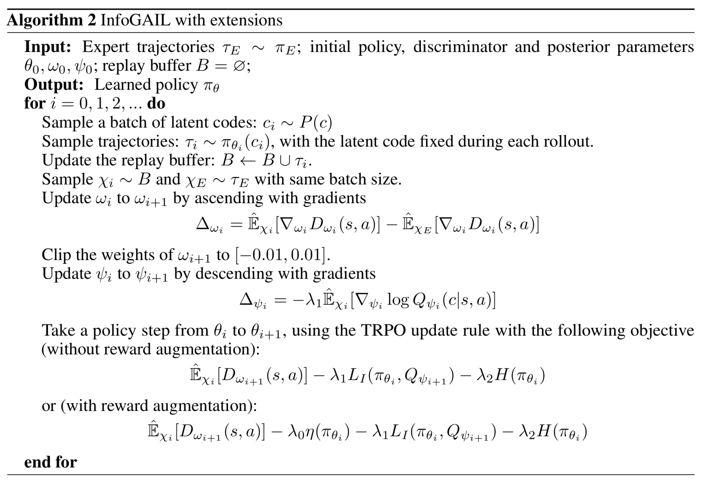
InfoGAIL
Modified GAIL
Objective Function
GAIL: \[ \underset{\pi}{\min} \underset{𝐷\in(0,1)^{S×A}}{\max} + 𝔼_{𝜋_𝐸} [ 𝑙𝑜𝑔(1 − 𝐷(𝑠, a))] − 𝜆𝐻(𝜋) \]
where 𝜋 is learner policy, and \(𝜋_𝐸\) is expert policy.
InfoGAIL:
- Discriminator: same with GAIL
- Generator: simply introducing latent factor c into 𝜋 → 𝜋 𝑎 𝑠, 𝑐
However, applying GAIL to 𝜋(𝑎 | 𝑠, 𝑐) could simply ignore c and fail to separate different expert behaviors → adding more constraints over c
Constraints over Latent Features
There should be high mutual information between the latent factor c and learner trajectory τ.
\[ I(c; \tau) = \sum_{\tau} p(\tau) \sum_c p(c|\tau) \log_2 \frac{p(c|\tau)}{p(c)} \]
Independence between c and trajectory τ:
\[ p(c|\tau) = \frac{p(c)p(\tau)}{p(\tau)}, \quad \frac{p(c|\tau)}{p(c)} = 1, \quad \log_2 \frac{p(c|\tau)}{p(c)} = 0 \]
Maximizing mutual information \(I(c; \tau)\)
→ hard to maximize directly as it requires the posterior \(P(c|\tau)\)
→ using \(Q(c|\tau)\) to estimate \(P(c|\tau)\) There should be high mutual information between the latent factor c and learner trajectory 𝜏.
Constraints over Latent Features
Introducing the lower bound \(L_I(\pi, Q)\) of \(I(c; \tau)\)
\[ \begin{align} & I(c; \tau) \\ &= H(c) - H(c|\tau) \\ &= \mathbb{E}_{a \sim \pi(\cdot|s,c)} \left[ \mathbb{E}_{c' \sim P(c|\tau)} [log P(c'|\tau)] \right] + H(c) \\ &= \mathbb{E}_{a \sim \pi(\cdot|s,c)} \left[ D_{KL}(P(\cdot|\tau) \| Q(\cdot|\tau)) + \mathbb{E}_{c' \sim P(c|\tau)} [log Q(c'|\tau)] \right] + H(c) \\ &\geq \mathbb{E}_{a \sim \pi(\cdot|s,c)} \left[ \mathbb{E}_{c' \sim P(c|\tau)} [log Q(c'|\tau)] \right] + H(c) \\ &= \mathbb{E}_{c \sim P(c), a \sim \pi(\cdot|s,c)} [log Q(c|\tau)] + H(c) \\ &= L_I(\pi, Q) \end{align} \]
Constraints over Latent Features
There should be high mutual information between the latent factor c and learner trajectory 𝜏.
Maximizing mutual information 𝐼(𝑐; 𝜏)
→ hard to maximize directly as it requires the posterior 𝑃(𝑐|𝜏)
→ using 𝑄(𝑐|𝜏) to estimate 𝑃(𝑐|𝜏)
Maximizing 𝐼(𝑐; 𝜏) through maximize the lower bound 𝐿𝐼(𝜋, 𝑄)
Objective Function
GAIL:
\[ \min_\pi \max_{D \in (0,1)^{S \times A}} \mathbb{E}_\pi [log D(s, a)] + \mathbb{E}_{\pi_E} [log(1 - D(s, a))] - \lambda H(\pi) \]
where \(\pi\) is learner policy, and \(\pi_E\) is expert policy.
InfoGAIL:
\[ \min_{\pi,Q} \max_D \mathbb{E}_\pi [log D(s, a)] + \mathbb{E}_{\pi_E} [log(1 - D(s, a))] - \lambda_1 L_I(\pi, Q) - \lambda_2 H(\pi) \]
\(\qquad \qquad \qquad \qquad \qquad \qquad\) where \(\lambda_1 > 0\) and \(\lambda_2 > 0\).
InfoGAIL
Additional Optimization
Improved Optimization
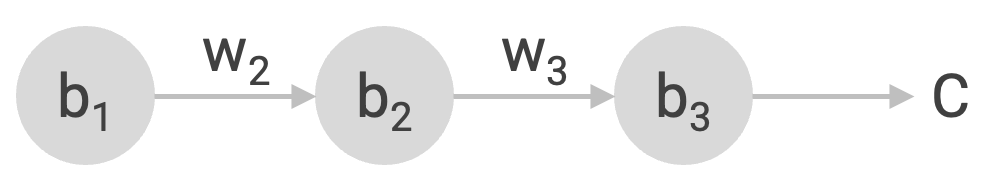
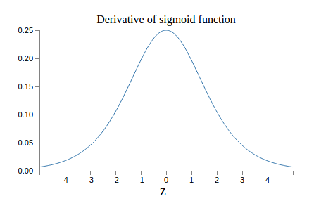
The traditional GAN objective suffers from vanishing gradient and mode collapse problems.
Vanishing gradient
\[ \frac{\partial C}{\partial b_1} = \frac{\partial C}{\partial y_3} \frac{\partial y_3}{\partial z_3} \frac{\partial z_3}{\partial x_3} \frac{\partial x_3}{\partial z_2} \frac{\partial z_2}{\partial x_2} \frac{\partial x_2}{\partial z_1} \frac{\partial z_1}{\partial b_1} \]
\[ = \frac{\partial C}{\partial y_{3}} \sigma'(z_{3}) w_{3} \sigma'(z_{2}) w_{2} \sigma'(z_{1}) \]
Improved Optimization
The traditional GAN objective suffers from vanishing gradient and mode collapse problems.
Mode collapse: generator tends to produce the same type of data → generator yields the same G(z) for different z
Improved Optimization
The traditional GAN objective suffers from vanishing gradient and mode collapse problems.
→ using the Wasserstein GAN (WGAN)
\[ \min_{\theta, \psi} \max_{\omega} \mathbb{E}_{\pi_\theta}[D_\omega(s, a)] - \mathbb{E}_{\pi_E}[D_\omega(s, a)] - \lambda_0 \eta(\pi_\theta) - \lambda_1 L_I(\pi_\theta, Q_\psi) - \lambda_2 H(\pi_\theta) \]
Experiments
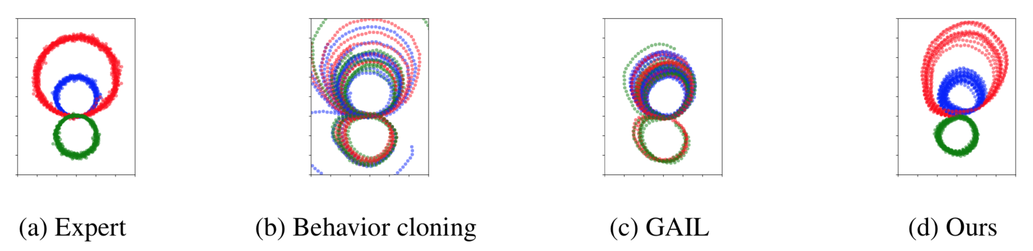
Learning to Distinguish Trajectories
- The observations at time t are positions from t − 4 to t.
- The latent code is a one-hot encoded vector with 3 dimensions and a uniform prior.
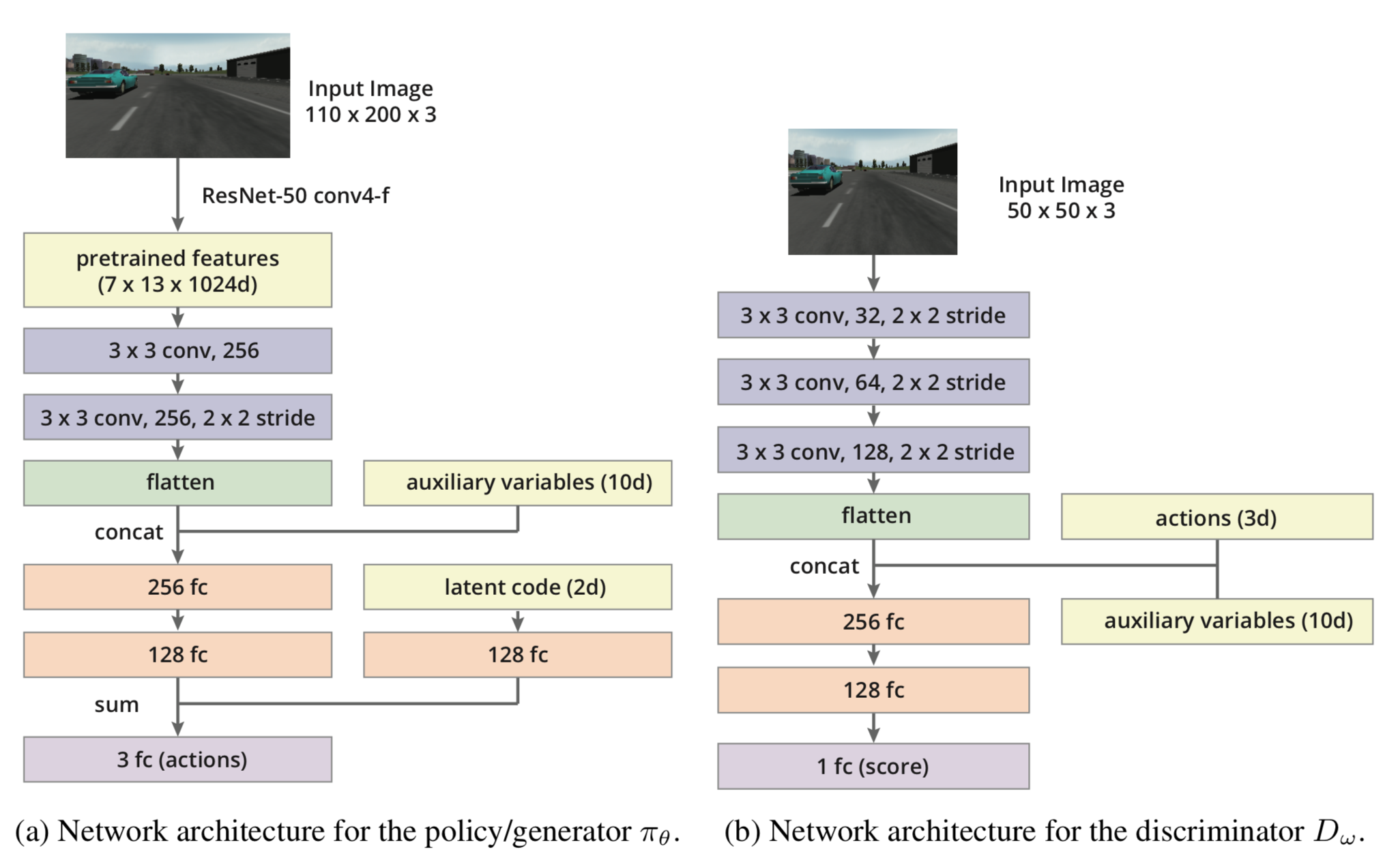
Self-driving car in the TORCS Environment
• The demonstrations collected by manually driving
• Three-dimensional continuous action composed of steering, acceleration,and braking
• Raw visual inputs as the only external inputs for the state
• Auxiliary information as internal input, including velocity at time t, actions at time t − 1 and t − 2, and damage of the car
• Pre-trained ResNet on ImageNet

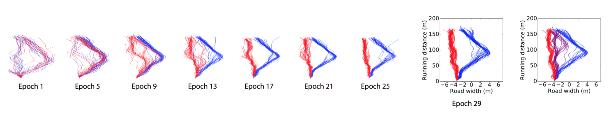
Performance
Turn
[0, 1] corresponds to using the inside lane (blue lines), while [1, 0] corresponds to the outside lane (red lines).
Performance
Pass
[0, 1] corresponds to passing from right (red lines), while [1, 0] corresponds to passing from left (blue lines).
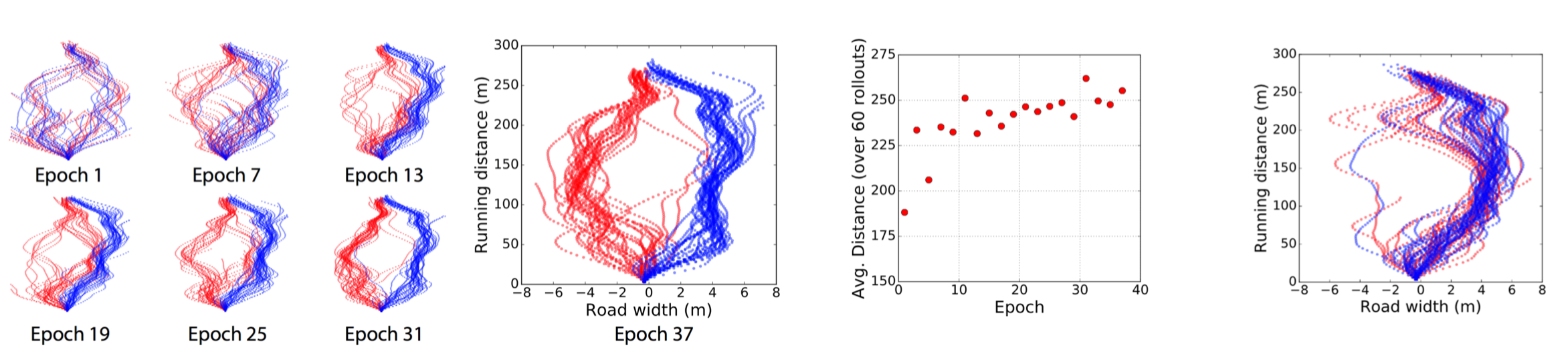
infoGAIL
GAIL
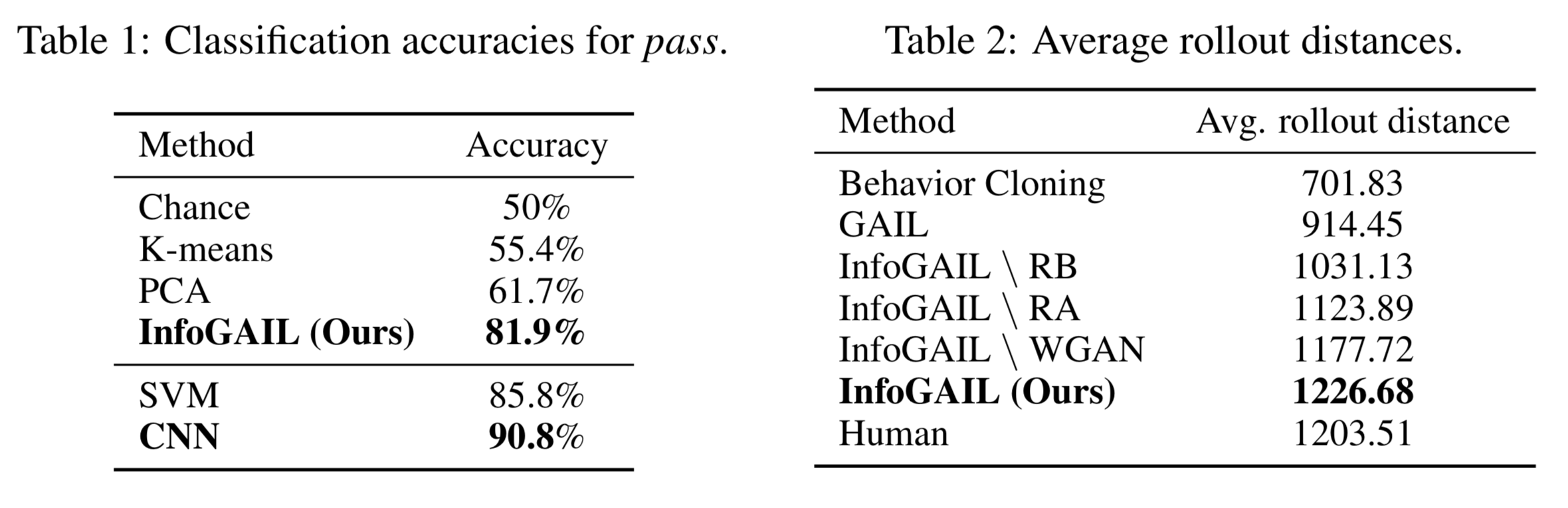
Performance
• Classification accuracies of 𝑄(𝑐|𝜏)
• Reward augmentation encouraging the car to drive faster
Today’s agenda
• Adversarial optimization for imitation learning (GAIL)
• Adversarial optimization with multiple inferred behaviors (InfoGAIL)
• Model based adversarial optimization (MGAIL)
• Multi-agent imitation learning
Model-based Adversarial Imitation Learning
Nir Baram, Oron Anschel, Shie Mannor
Presented by Yuwen Xiong, Mar 1 st
Recap: GAIL algorithm
\[ \underset{\pi}{\text{argmin}} \quad \underset{D \in (0,1)}{\text{argmax}} \mathbb{E}_{\pi}[\log D(s, a)] + \mathbb{E}_{\pi_E}[\log(1 - D(s, a))] - \lambda H(\pi) \]
- We use Adam to optimize the discriminator and use TRPO to optimize the policy
- The optimization of the discriminator can be done by using backpropagation, but this is not the case for the optimization of the policy
- \(\pi\) affects the data distribution but do not appear in the objective itself
- We use these two equations to get gradient estimation for \(\pi_{\theta}\)
\[ \nabla_{\theta} \mathbb{E}_{\pi}[\log D(s, a)] \cong \mathbb{\hat{E}}_{\tau_i}[\nabla_{\theta} \log \pi_{\theta}(a|s) Q(s, a)] \]
\[Q(\hat{s}, \hat{a}) = \mathbb{\hat{E}}_{\tau_i}[\log D(s, a) \mid s_0 = \hat{s}, a_0 = \hat{a}]\]
Motivation
- A model-free approach like GAIL has its limitations
- The generative model can no longer be trained by simply backpropagating the gradient from the loss function defined over the discriminator
- Has to resort to high-variance gradient estimations
- If we have a model-based version of adversarial imitation learning
- The system can be easily trained end-to-end using regular backpropagation
- The policy gradient can be derived directly from the gradient of the discriminator
- Policies can be more robust and training requires fewer interactions with the environment
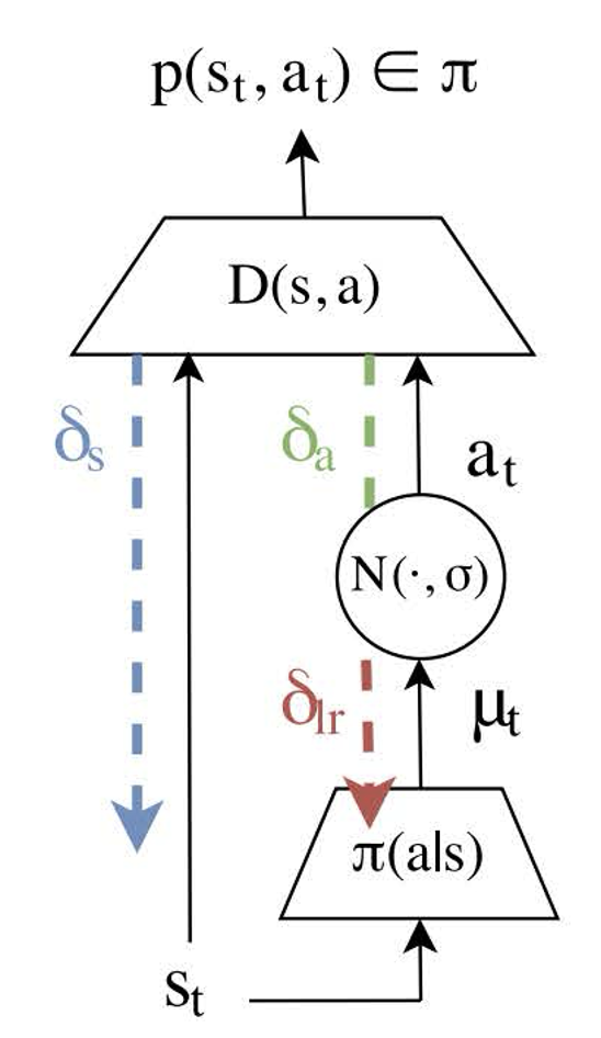
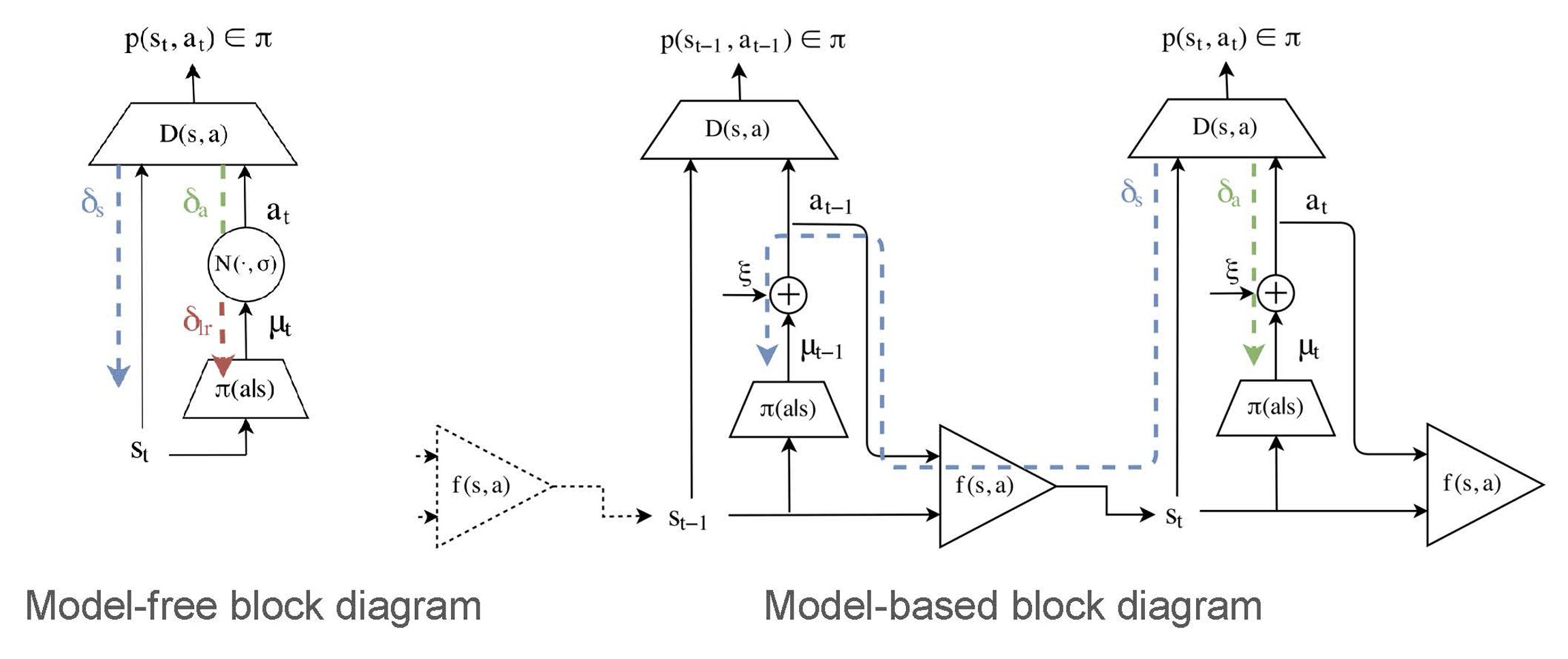
Algorithm - overview
The model-free approach treats the state s as fixed and only tries to optimize the behavior.
Instead, we treat s as a function of the policy: \[s' = f(s, a)\]
So that, by using the law of total derivative we can get:
\[ \begin{align} \left.\nabla_{\theta} D(s_t, a_t)\right|_{s=s_t, a=a_t} &= \left.\frac{\partial D}{\partial a} \frac{\partial a}{\partial \theta}\right|_{a=a_t} + \left.\frac{\partial D}{\partial s} \frac{\partial s}{\partial \theta}\right|_{s=s_t} \\ &= \left.\frac{\partial D}{\partial a} \frac{\partial a}{\partial \theta}\right|_{a=a_t} + \frac{\partial D}{\partial s} \left(\left.\frac{\partial f}{\partial s} \frac{\partial s}{\partial \theta}\right|_{s=s_{t-1}} + \left.\frac{\partial f}{\partial a} \frac{\partial a}{\partial \theta}\right|_{a=a_{t-1}}\right) \end{align} \]
Algorithm - preparation
First, we know that \(D(s, a) = p(y|s, a)\), where \(y = \{\pi_E, \pi\}\)
By using Bayes rule and the law of total probability we can get:
\[D(s, a) = p(\pi|s, a) = \frac{p(s, a|\pi)p(\pi)}{p(s, a)}\]
\[\qquad \qquad \qquad = \frac{p(s, a|\pi)p(\pi)}{p(s, a|\pi)p(\pi) + p(s, a|\pi_E)p(\pi_E)}\]
\[\qquad = \frac{p(s, a|\pi)}{p(s, a|\pi) + p(s, a|\pi_E)}\]
Algorithm - preparation
Re-writing it as following:
\[ D(s, a) = \frac{1}{\frac{p(s,a|\pi)+p(s,a|\pi_E)}{p(s,a|\pi)}} = \frac{1}{1 + \frac{p(s,a|\pi_E)}{p(s,a|\pi)}} = \frac{1}{1 + \frac{p(a|s,\pi_E)}{p(a|s,\pi)} \cdot \frac{p(s|\pi_E)}{p(s|\pi)}}\]
Let \(\varphi(s, a) = \frac{p(a|s,\pi_E)}{p(a|s,\pi)}\) and \(\psi(s) = \frac{p(s|\pi_E)}{p(s|\pi)}\), we can get:
\[ D(s, a) = \frac{1}{1 + \varphi(s, a) \cdot \psi(s)} \]
Algorithm - preparation
Here \(\varphi(s, a) = \frac{p(a|s,\pi_E)}{p(a|s,\pi)}\) stands for policy likelihood ratio
And \(\psi(s) = \frac{p(s|\pi_E)}{p(s|\pi)}\) stands for state distribution likelihood ratio
By using differentiation rule we can easily get:
\[ \nabla_a D = -\frac{\varphi_a(s, a)\psi(s)}{(1 + \varphi(s, a)\psi(s))^2} \]
\[ \nabla_s D = -\frac{\varphi_s(s, a)\psi(s) + \varphi(s, a)\psi_s(s)}{(1 + \varphi(s, a)\psi(s))^2} \]
Recall what we need: \(\left.\nabla_\theta D(s_t, a_t)\right|_{s=s_t,a=a_t} = \left.\frac{\partial D}{\partial a} \frac{\partial a}{\partial \theta}\right|_{a=a_t} + \left.\frac{\partial D}{\partial s} \frac{\partial s}{\partial \theta}\right|_{s=s_t}\)
Algorithm - re-parameterization of distribution
Assuming the policy is given by
\[ \pi_\theta(a|s) = \mathcal{N}(a|\mu_\theta(s), \sigma_\theta^2(s)) \]
We can rewrite it to
\[ \pi_\theta(a|s) = \mu_\theta(s) + \xi\sigma_\theta(s), \text{ where } \xi \sim \mathcal{N}(0, 1) \]
So that we can get a Monte-Carlo estimator of the derivative
\[ \begin{align} \nabla_\theta \mathbb{E}_\pi(a|s) D(s, a) &= \mathbb{E}_{\rho(\xi)} \nabla_a D(a, s) \nabla_\theta \pi_\theta(a|s) \\ & \cong \frac{1}{M} \sum_{i=1}^M \left.\nabla_a D(s, a) \nabla_\theta \pi_\theta(a|s)\right|_{\xi=\xi_i} \end{align} \]
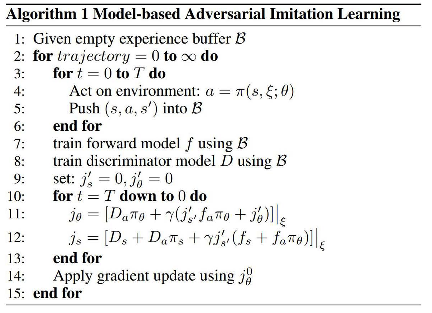
Algorithm
Algorithm
To maximize the reward function, we can view reward as \(r(s, a) = -D(s, a)\), and then maximizing the total reward is equivalent to minimizing the total discriminator beliefs along a trajectory.
So that we can define: \[ J(\theta) = \mathbb{E} \left[ \sum_{t=0} \gamma^t D(s_t, a_t) \mid \theta \right] \]
And write down the derivatives: (this follows SVG paper [Heess et al. 2015]) \[ J_s = \mathbb{E}_{p(a\mid s)}\mathbb{E}_{p(s'\mid s,a)}\mathbb{E}_{p(\xi\mid s,a,s')} \left[ D_s + D_a\pi_s + \gamma J'_{s'}(f_s + f_a\pi_s) \right] \]
\[ J_\theta = \mathbb{E}_{p(a\mid s)}\mathbb{E}_{p(s'\mid s,a)}\mathbb{E}_{p(\xi\mid s,a,s')} [D_a\pi_\theta + \gamma(J'_{s'}f_a\pi_\theta + J'_\theta)] \]
Algorithm
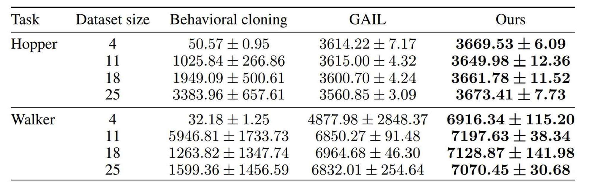
Experiments
Today’s agenda
• Adversarial optimization for imitation learning (GAIL)
• Adversarial optimization with multiple inferred behaviors (InfoGAIL)
• Model based adversarial optimization (MGAIL)
• Multi-agent imitation learning