CSC2626 Imitation Learning for Robotics
Week 7: Imitation as Program Induction and Modular Decomposition of Demonstrations
Today’s agenda
• Learning programs based on execution traces (NPI - Neural Programmer Interpreters)
• Extending NPI for video-based robot imitation (NTP - Neural Task Programming)
• Inferring sub-task boundaries (TACO - Temporal Alignment for Control)
• Learning to search in Task and Motion Planning (TAMP)
• Generalization through imitation – using hierarchical policies
Neural Programmer-Interpreters
By Scott Reed & Nando de Freitas
Motivation
Neural Programmer-Interpreters (NPI) is an attempt to use neural methods to train machines to carry out simple tasks based on a small amount of training data.
Recurrent neural network (RNN)
![]()
• RNN is a neural network with feedback
• Hidden state is to capture history information and current state of the network
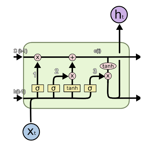
Long Short Term Memory (LSTM)
• LSTM is a special kind of RNN
• Gates are used to control information flow. Just like a valve
Model
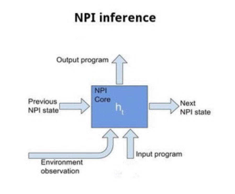
• The NPI core is a LSTM network that learns to represent and execute programs given their execution traces
![]()
NPI core module
![]()
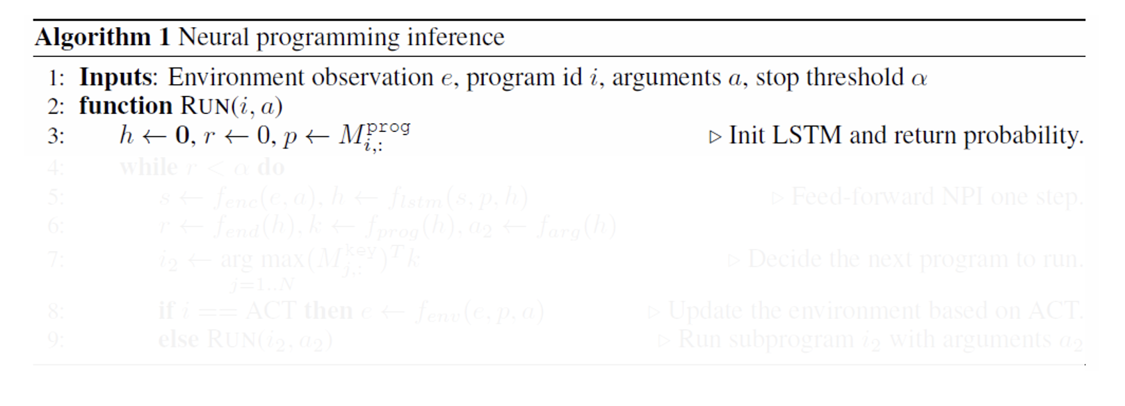
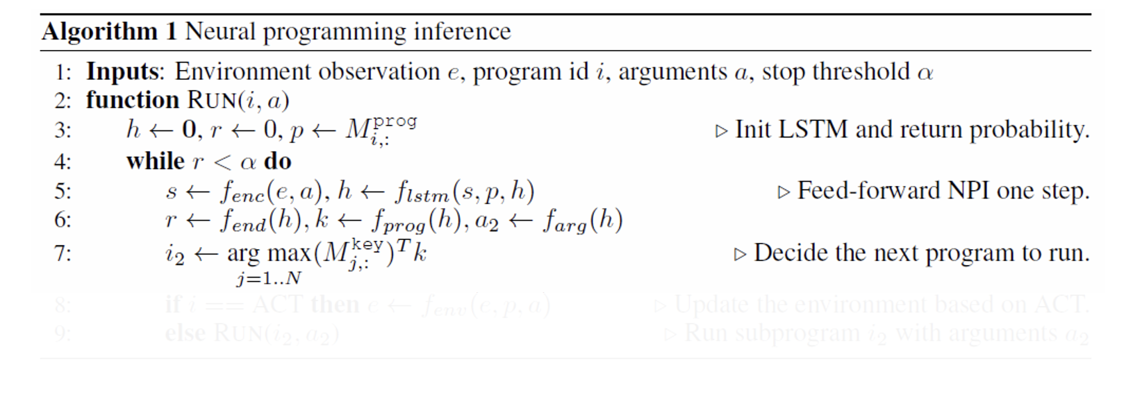
Algorithm - inference
![]()
Line 3: \(𝑀^{𝑝𝑟𝑜𝑔}\) and \(𝑀^{𝑘𝑒𝑦}\) are memory banks to store program embeddings and program keys
Algorithm - inference
![]()
Line 7: \((𝑀_{𝑗,}^{𝑘𝑒𝑦})^{𝑇}𝑘\) is directly measurement for cosine similarity
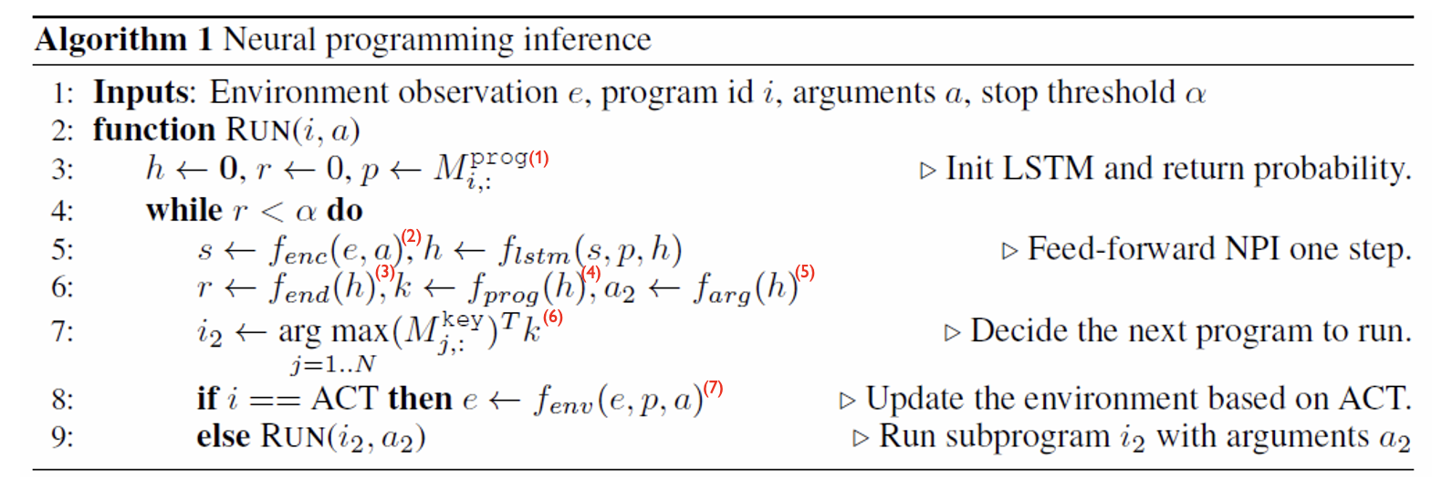
Algorithm - inference
![]()
(1): \(𝑀^{𝑝𝑟𝑜𝑔}\) and \(𝑀^{𝑘𝑒𝑦}\) are memory storing program embeddings and program keys
(2): \(𝑓_{𝑒𝑛𝑐}\) is a domain-specific encoder (for different tasks, have different encoders)
(3): \(𝑓_{𝑒𝑛𝑑}\) is to calculate the probability of finishing the program
(4): \(𝑓_{𝑝𝑟𝑜𝑔}\) is to retrieve the next program key from memory
(5): \(𝑓_{𝑎𝑟𝑔}\) is to return the next program’s arguments
(6): \((𝑀_{𝑗,}^{𝑘𝑒𝑦})^{𝑇}𝑘\) is to measure cosine similarity
(7): \(𝑓_{env}\) is a domain-specific transition mapping
Training
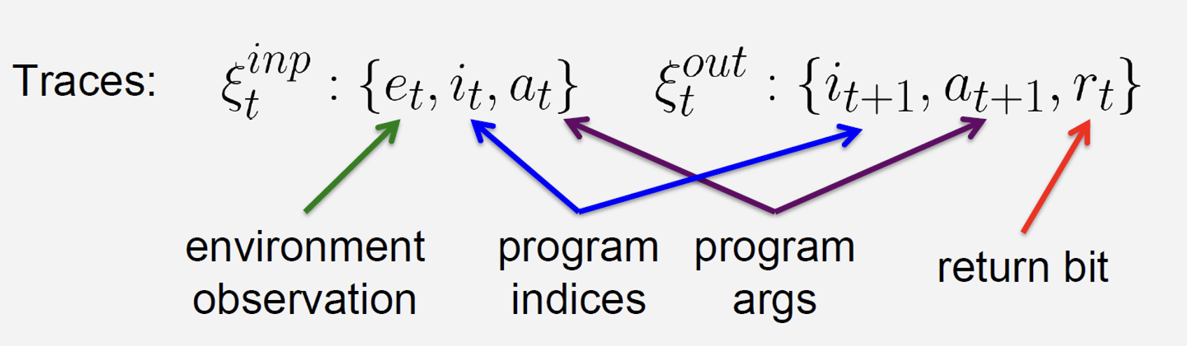
Directly maximize the probability of the correct execution trace output \(𝞷^{𝑜𝑢𝑡}\) conditioned on \(𝞷^{𝑖𝑛𝑝}\):
\[
𝜃^∗ = 𝑎𝑟𝑔 \underset{𝜃}{max} \sum_{(𝞷^{𝑖𝑛𝑝}, 𝞷^{𝑜𝑢𝑡})} 𝑙𝑜𝑔𝑃(𝞷^{𝑜𝑢𝑡}|𝞷^{𝑖𝑛𝑝}, 𝜃)
\]
Then we can just run gradient ascent to optimize it
Tasks
• Addition
• Teach the model the standard grade school algorithm of adding 2 base-10 numbers
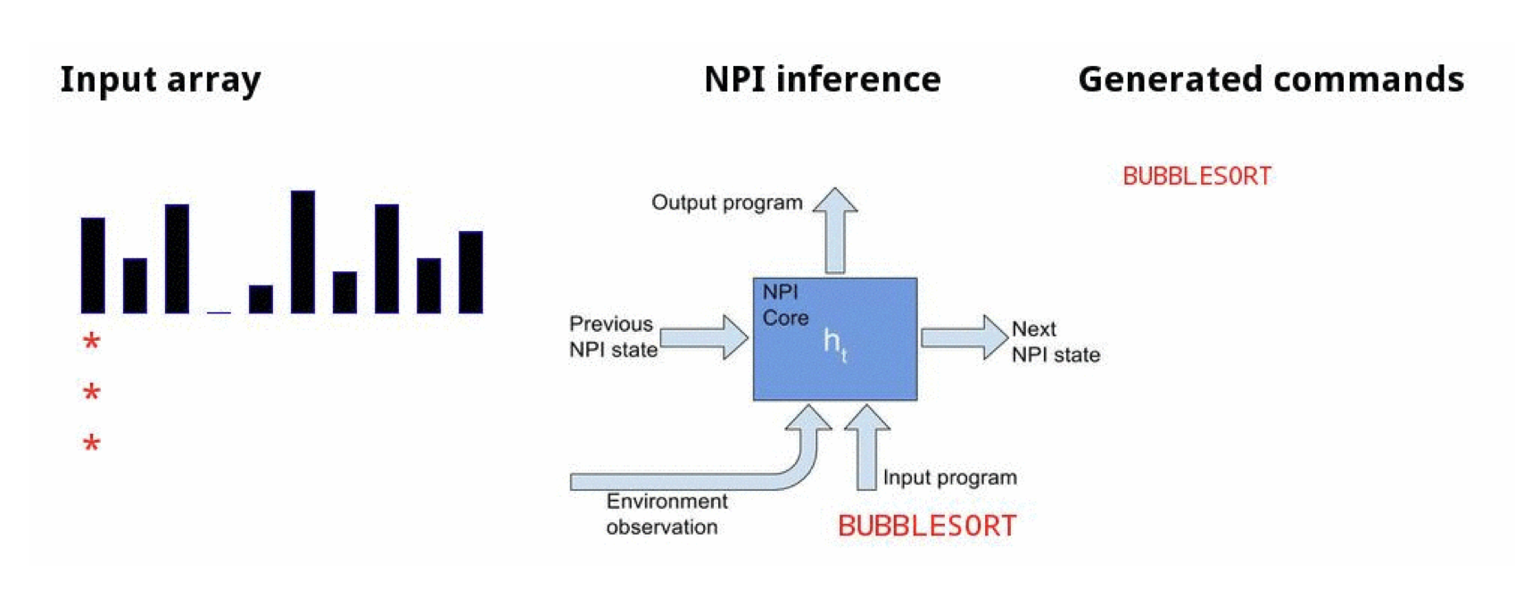
• Sorting
• Teach the model bubble sorting to sort an array of numbers in ascending order
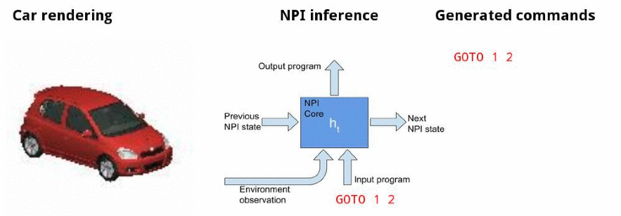
• Canonicalizing 3D models
• Teach the model to generate a trajectory of actions that delivers the camera to the target view, e.g, frontal pose at a 15° elevation
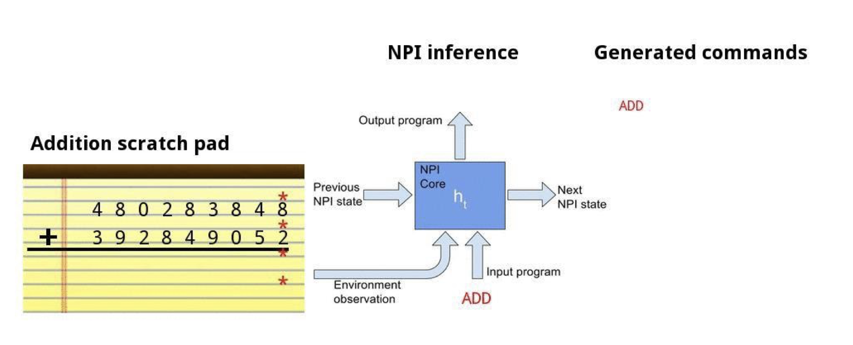
Adding numbers together
![]()
Addition demo
![]()
Bubble sort
![]()
Sorting demo
![]()
Canonicalizing 3D models
![]()
Canonicalizing demo
![]()
Experiments
• Data Efficiency
• Generalization
• Learning new programs with a fixed NPI cores
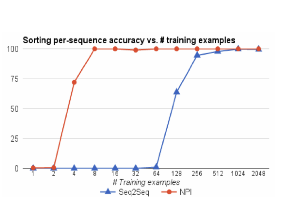
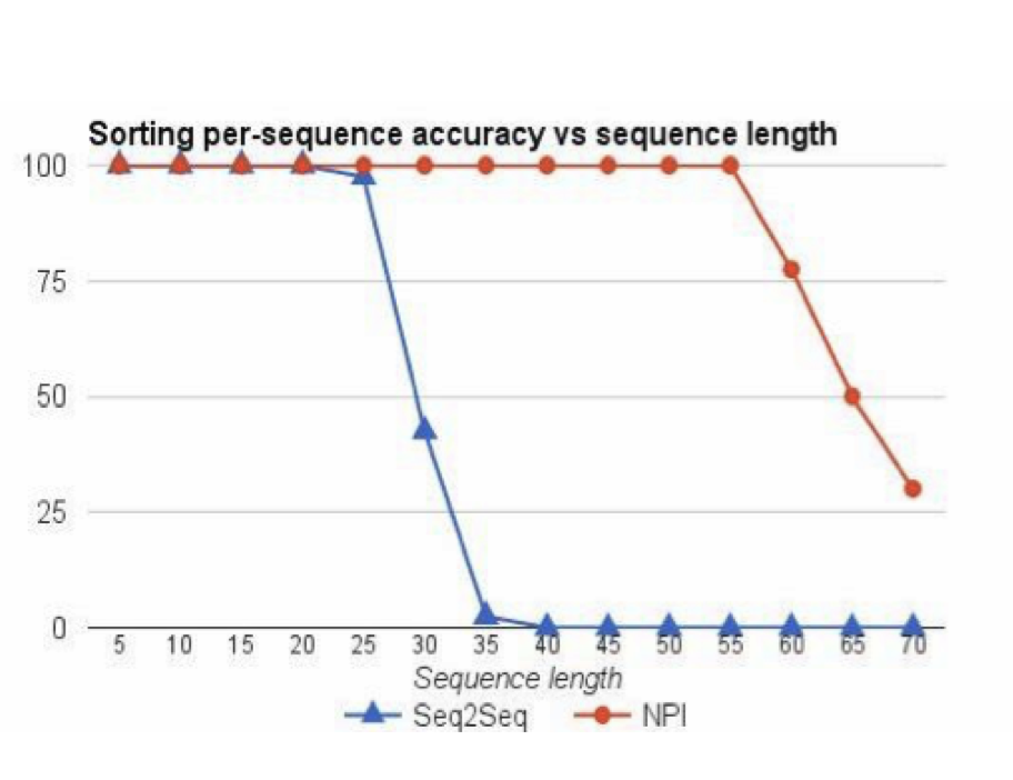
Data Efficiency - Sorting
• Seq2Seq LSTM and NPI used the same number of layers and hidden units.
• Trained on length up to 20 arrays of single-digit numbers.
• NPI benefits from mining multiple subprogram examples per sorting instance, and additional parameters of the program memory.
Generalization - Sorting
• For each length up to 20, they provided 64 example bubble sort traces, for a total of 1216 examples.
• Then, they evaluated whether the network can learn to sort arrays beyond length 20
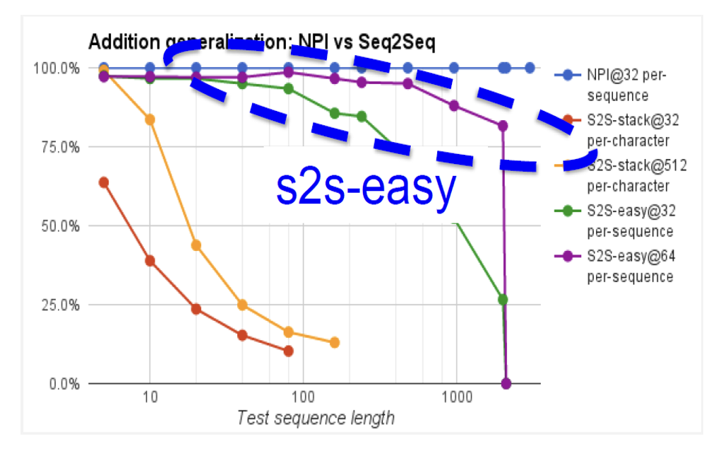
Generalization - Adding
• NPI trained on 32 examples for sequence length up to 20
• s2s-easy trained on twice as many examples as NPI (purple curve)
• s2s-stack trained on 16 times more examples than NPI (orange curve)
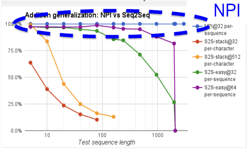
Generalization - Adding
• NPI trained on 32 examples for sequence length up to 20
• s2s-easy trained on twice as many examples as NPI (purple curve)
• s2s-stack trained on 16 times more examples than NPI (orange curve)
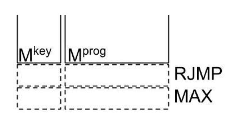
Learning New Programs with a Fixed NPI Core
• Toy example: maximum-finding in an array
• Simple (not optimal) way: call BUBBLESORT and then take the right-most element of the array. Two new programs:
• RJMP: Move all pointers to the rightmost position in the array by repeatedly calling RSHIFT program
• MAX: Call BUBBLESORT and then RJMP
• Expand program memory by adding 2 slots. Then learn by backpropagation with the NPI core and all other parameters fixed.
Learning New Programs with a Fixed NPI Core
Only the memory slots of
the new program are updated!
All other weights are
fixed!
Protocol:
• Randomly initialize new program vectors in memory
• Freeze core and other program vectors
• Backpropagate gradients to new program vectors
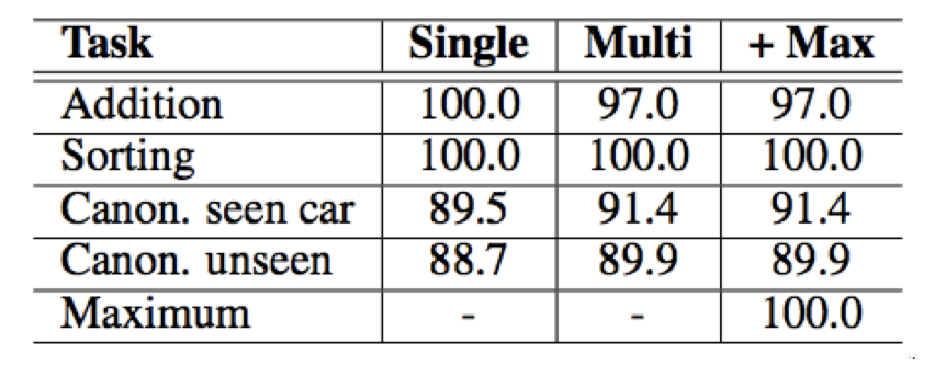
Quantitative Results
• Numbers are per-sequence % accuracy
• + Max: indicates performance after addition of MAX program to memory
• “unseen” uses a test set with disjoint car models from the training set
Today’s agenda
• Learning programs based on execution traces (NPI - Neural Programmer Interpreters)
• Extending NPI for video-based robot imitation (NTP - Neural Task Programming)
• Inferring sub-task boundaries (TACO - Temporal Alignment for Control)
• Learning to search in Task and Motion Planning (TAMP)
• Generalization through imitation – using hierarchical policies
Neural Task Programming: Learning to Generalize Across Hierarchical Tasks
Danfei Xu, Suraj Nair, Yuke Zhu, Julian Gao, Animesh Garg, Li Fei-Fei, Silvio Savarese
Presented by Angran Li
February 8, 2019
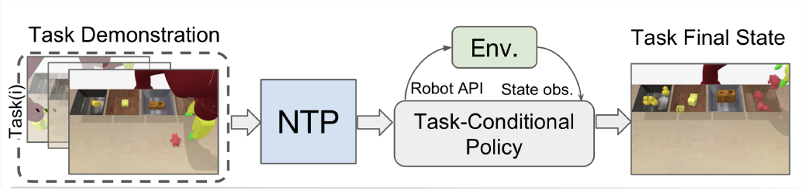
How the Algorithm works?
![]()
- Task Demonstration: state trajectory, first/third-person video demonstrations, or a list of language instructions.
- Task-Conditional Policy: a neural program.
- Using callable primitive actions to interact with the environment.
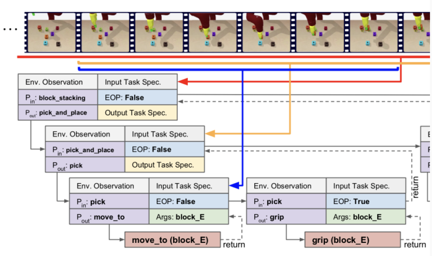
How the Algorithm works?
![]()
Top-level program block_stacking is recursively decomposed to bottom-level API move_to and grip.
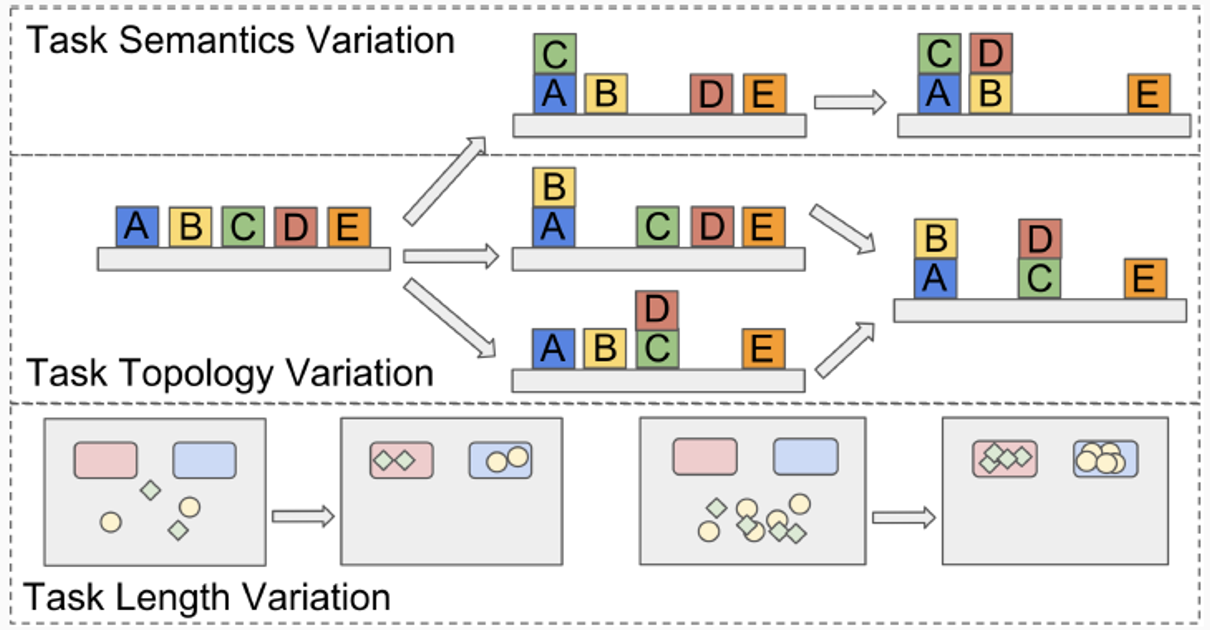
Goals
Learning to Generalize Across Hierarchical Tasks
- Generalizing the learned policies to new task objectives
- Task Length: more objects to transport
- Task Semantics: a different goal
- Task Topology: a different trajectory to the same goal
- Hierarchical composition of primitive actions
- Modularization and reusability
- Learn the latent structure in complex tasks, instead of fake dependencies
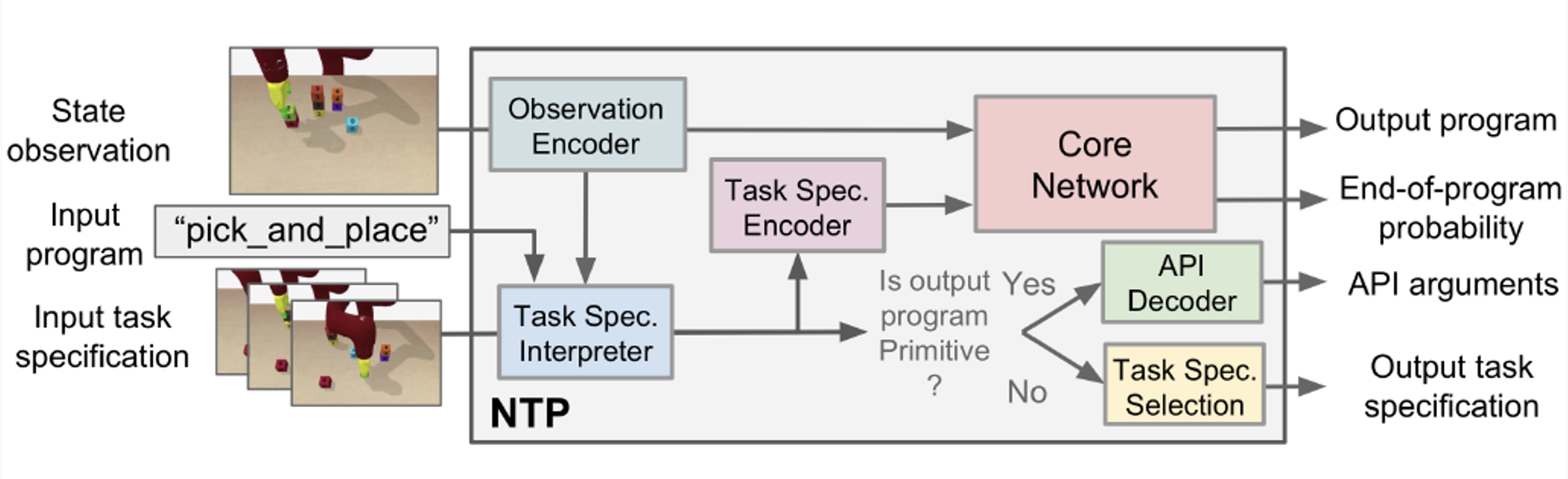
Implementation: Neural Task Programming
![]()
- Observation Encoder: observation \(o_i \Rightarrow\) state representation \(s_i\)
- Task Spec. Interpreter: \(\Rightarrow\) API arguments \(a_i\) or task spec. \(\psi_{i+1}\)
- Task Spec. Encoder: task spec. \(\psi_i \Rightarrow\) vector space \(\phi_i\)
- Core Network: \(s_i, P_i, \phi_i \Rightarrow P_{i+1}, r_i\)
Implementation: Standing on the shoulder of NPI
Neural Task Programming combines the idea of Few-Shot Learning from Demonstration and Neural Programmer-Interpreters.
- Similarities when executing a program:
- When the EOP probability exceeds a threshold \(\alpha\), control is returned to the caller program;
- When the program is not primitive, a sub-program with its arguments is called;
- When the program is primitive, a low-level basic action is performed.
- Two similar modules:
- Domain-specific task encoders that map an observation to a state representation.
- A key-value memory that stores and retrieves program embeddings.
Implementation: NTP vs NPI
- NPI: one-shot generalization to tasks with longer lengths; can’t generalizing to novel programs without training.
- NTP: generalizes to sub-task permutations (topology) and success conditions (semantics).
- Three main differences of NTP than the original NPI:
- NTP can interpret task specifications and perform hierarchical decomposition and thus can be considered as a meta-policy;
- It uses robot APls as the primitive actions to scale up neural programs for complex tasks;
- It uses a reactive core network instead of a recurrent network, making the model less history-dependent, enabling feedback control for recovery from failures.
Model Training
The model is trained using rich supervision from program execution traces \(\{\xi_t| \xi_t = (\Psi_t, p_t, s_t), t = 1 \ldots T\}\).
The training objective is to maximize the probability of the correct executions over all the tasks in the dataset \(D = \{(\xi_t, \xi_{t+1})\}\).
For each task specification, the ground-truth hierarchical decomposition is provided by the expert policy, which is an agent with hard-coded rules.
Experiments: Setup
![]()
- Generalization in 3 variations: semantics, topology, and length.
- Using image-based input without access to ground truth state.
- Working in real-world tasks combine these variations.
→ Three tasks: Object Sorting, Block Stacking, and Table Clean-up
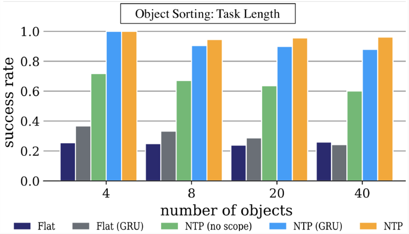
Experiments: Object Sorting
![]()
Flat: non-hierarchical model, directly predicts the primitive APls instead of calling hierarchical programs.
GRU: Gated Recurrent Unit.
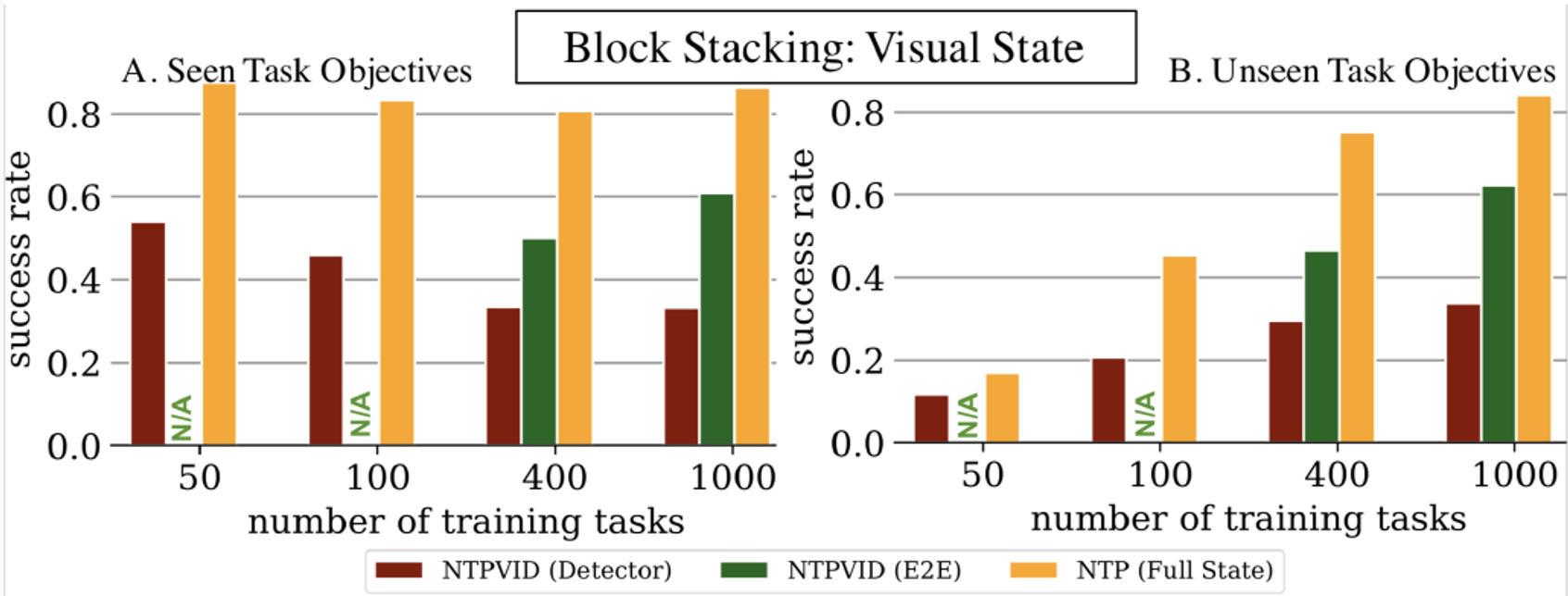
Experiments: Block Stacking
![]()
- NTPVID(E2E): Trained with only visual information.
- NTP(Full State): Trained with ground-truth hierarchical decomposition.
Experiments: Table Clean-up
![]()
Discussion & Future Work
- Neural Task Programming:
- A meta-learning framework that learns modular and reusable neural programs for hierarchical tasks.
- Generalizing well towards the variation of task length, semantics, and topology for complex tasks.
- Future work:
- Improve the state encoder to extract more task-salient information such as object relationships;
- Devise a richer set of APls such as velocity and torque-based controllers;
- Extend this framework to tackle more complex tasks on real robots.
Today’s agenda
• Learning programs based on execution traces (NPI - Neural Programmer Interpreters)
• Extending NPI for video-based robot imitation (NTP - Neural Task Programming)
• Inferring sub-task boundaries (TACO - Temporal Alignment for Control)
• Learning to search in Task and Motion Planning (TAMP)
• Generalization through imitation – using hierarchical policies
TACO: Learning Task Decomposition via Temporal Alignment for Control
Kyriacos Shiarlis, Markus Wulfmeier, Sasha Salter, Shimon Whiteson, Ingmar Posner
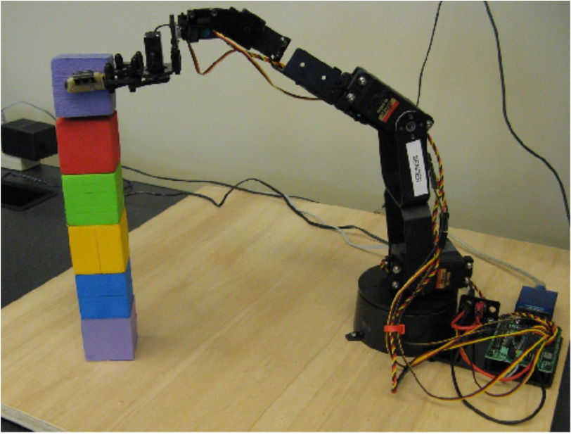
Motivation – Block Stacking Task
Complex tasks can often be broken down into simpler sub-tasks
Most Learning from Demonstration (LfD) algorithms can only learn a single policy for the whole task
Resulting in more complex policies, and also less reusable
Modular LfD
Modelling the task as a composition of sub-tasks
Reusable sub-policies (modules) are learned for each sub-task.
Sub-policies are easier to learn and can be composed in different ways to execute new tasks.
Key approach: provide the learner with additional information about the demonstration
TACO: Temporal Alignment for Control
- Partly supervised
- Domain agnostic
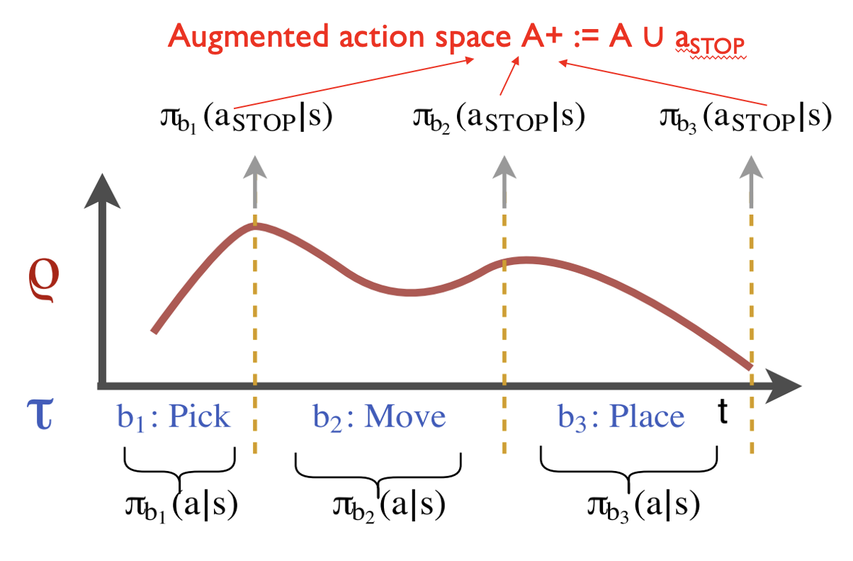
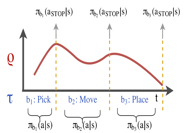
- Demonstration is augmented by task sketches - a sequence of sub-tasks that occur within the demonstration
\[
𝛕 = (b1, b2, . . . , bL),
\]
- Simultaneously aligns the sketches with the observed demonstrations and learns the required sub-policies
Example: Block stacking task
![]()
Problem
How to align task-sketches with the demonstration?
Solution: Borrow temporal sequence alignment techniques from speech recognition!
TACO: Temporal Alignment for Control
𝛕 = (b1, b2, . . . , bL),
Input sequence ρ with length T
A path \(ζ = (ζ_1, ζ_2, ..., ζ_T )\) is a sequence of sub- tasks of the same length as the input sequence ρ, describing the active sub-task \(ζ_t\) at every time-step
\(Z_{T,𝛕}\) is the set of all possible paths of length T for a task sketch 𝛕
Eg. T = 6, 𝛕 = (b1, b2, b3), ζ = (b1, b1, b2, b3, b3, b3)
TACO: Temporal Alignment for Control
Objective: Maximise the joint log likelihood of the task sequence and the actions conditioned on the states
\[
p(\tau, \mathbf{a}_\rho \mid s_\rho) = \sum_{\zeta \in \mathbb{Z}_{T, \tau}} p(\zeta \mid s_\rho) \prod_{t=1}^{T} \pi_{\theta_{\zeta_t}} (a_t \mid s_t)
\]
\(p(ζ |s_ρ)\) is the product of the stop, \(a_{STOP}\) , and nonstop, \(ā_{STOP}\), probabilities associated with any given path.
Eg. T = 4, \(s_⍴ = (s_0, s_1, s_2, s_3)\), 𝛕 = (b1, b2), ζ = (b1, b1, b2, b2)
\(p(ζ |sρ) = π_{b1}(non-stop)^* π_{b1}(stop)^* π_{b2}(non-stop)^* π_{b2}(stop)\)
TACO: Temporal Alignment for Control
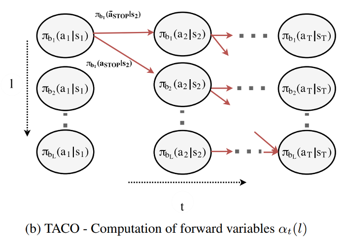
Problem: Impossible to compute all paths ζ in \(Z_{T,tau}\) for long sequence
Solution: Dynamic Programming
The (joint) likelihood of a being at sub-task l at time t can be formulated in terms of forward variables:
\[
\alpha_t(l) := \sum_{\zeta_{1:t} \in \mathbb{Z}_t, \tau_{1:l}} p(\zeta \mid s_\rho) \prod_{t' = 1}^{t} \pi_{\theta_{\zeta_{t'}}}(a_{t'} \mid s_{t'})
\]
TACO: Temporal Alignment for Control
\(\alpha_1(l) = \begin{cases}
\pi_{\theta_{b_1}}(a_1|s_1), & \text{if } l = 1, \\
0, & \text{otherwise}.
\end{cases}\)
\(\alpha_t(l) = \pi_{\theta_{b_l}}(a_t|s_t) \left[ \alpha_{t-1}(l-1) \pi_{\theta_{b_{l-1}}}(a_{STOP}|s_t) \right.\)
\(\left. + \alpha_{t-1}(l)(1 - \pi_{\theta_{b_l}}(a_{STOP}|s_t)) \right].\)
\(\alpha_T(L) = p(\tau, \mathbf{a}_\rho|\mathbf{s}_\rho).\)
Training: Maximize \(⍺_T(L)\) over θ
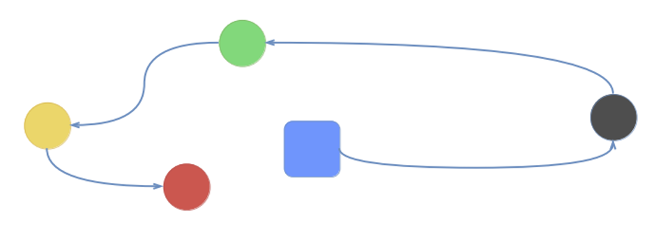
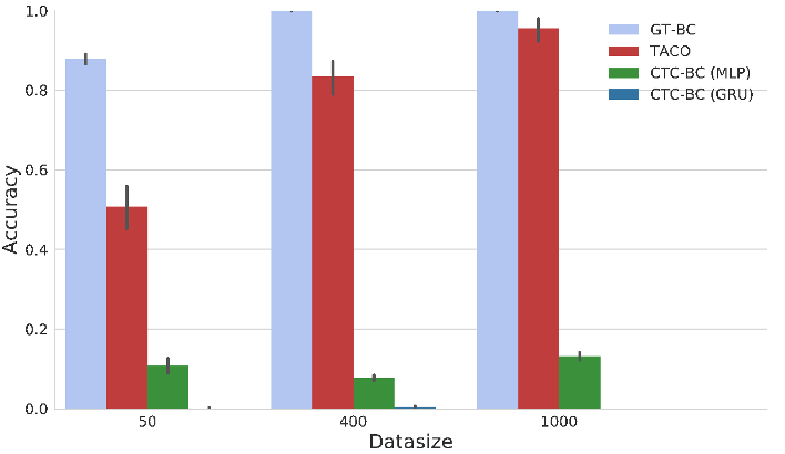
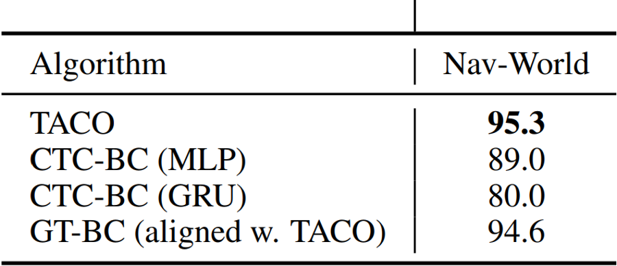
Experiments: Nav-World
Setup:
- The agent (blue) receives a route as a task sketch.
- 𝛕 = (black, green, yellow, red)
- State space: (x, y) distance from each of the destination points
- Action space: \((v_x, v_y)\) - the velocity
Training:
- Provided with state-action trajectories ⍴ and the task sketch.
- At the end of learning, the agent learns four sub-policies
![]()
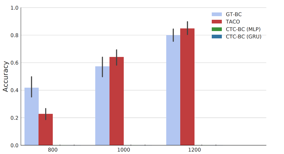
Test:
- Given an unseen task sketch.
- Considered successful if the agent visits all destinations in the correct order
Summary: TACO - Temporal Alignment for Control
Future Work & Limitation
Limitation:
- Sub-tasks in the task sketch has to be placed in the correct order
Future work:
Today’s agenda
• Learning programs based on execution traces (NPI - Neural Programmer Interpreters)
• Extending NPI for video-based robot imitation (NTP - Neural Task Programming)
• Inferring sub-task boundaries (TACO - Temporal Alignment for Control)
• Learning to search in Task and Motion Planning (TAMP)
• Generalization through imitation – using hierarchical policies
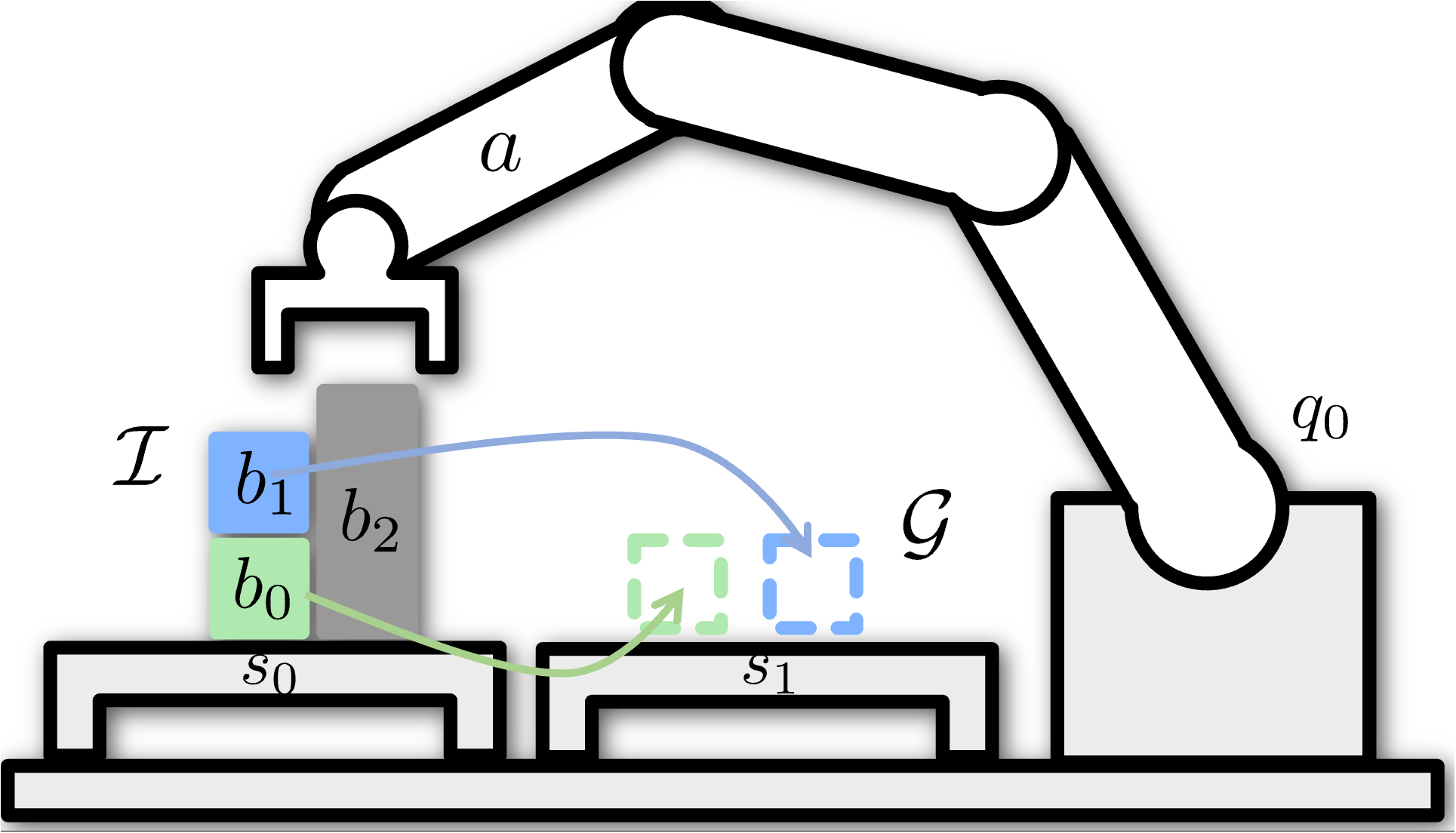
Task and Motion Planning
Goal: move green box and blue box on the goal surface
Problem: grey box is obstructing
Task plan:
- move grey box where it doesn’t obstruct
- move blue box on goal surface
- move green box on goal surface
Task and Motion Planning
![]()
Discrete action space: 3 objects x 4 operations
Continuous action space: 5 joint angles on the robot arm x T timesteps
find-grasp(b, hand)
place(b, hand, sur face)
find-traj(hand, goal)
collides(arm, b, objects)
\(b \in \{b_0, b_1, b_2 \}\)
Task and Motion Planning
![]()
Discrete action space: M objects x N operations
Continuous action space: 5 joint angles on the robot arm x T timesteps
find-grasp(b, hand)
place(b, hand, sur face)
find-traj(hand, goal)
collides(arm, b, objects)
pour(b, b’)
stir(b)
shake(b)
.
.
.
Task and Motion Planning
![]()
Discrete action space: M objects x N operations
Continuous action space: 5 joint angles on the robot arm x T timesteps
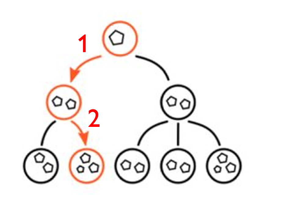
Discrete + Continuous Optimization
![]()
Expanding 1 and 2 requires solving continuous optimization problems with constraints
These plans are useful, but unfortunately discrete + continuous optimization is slow
Q: How can we learn to plan from past experience of having solved similar problems?
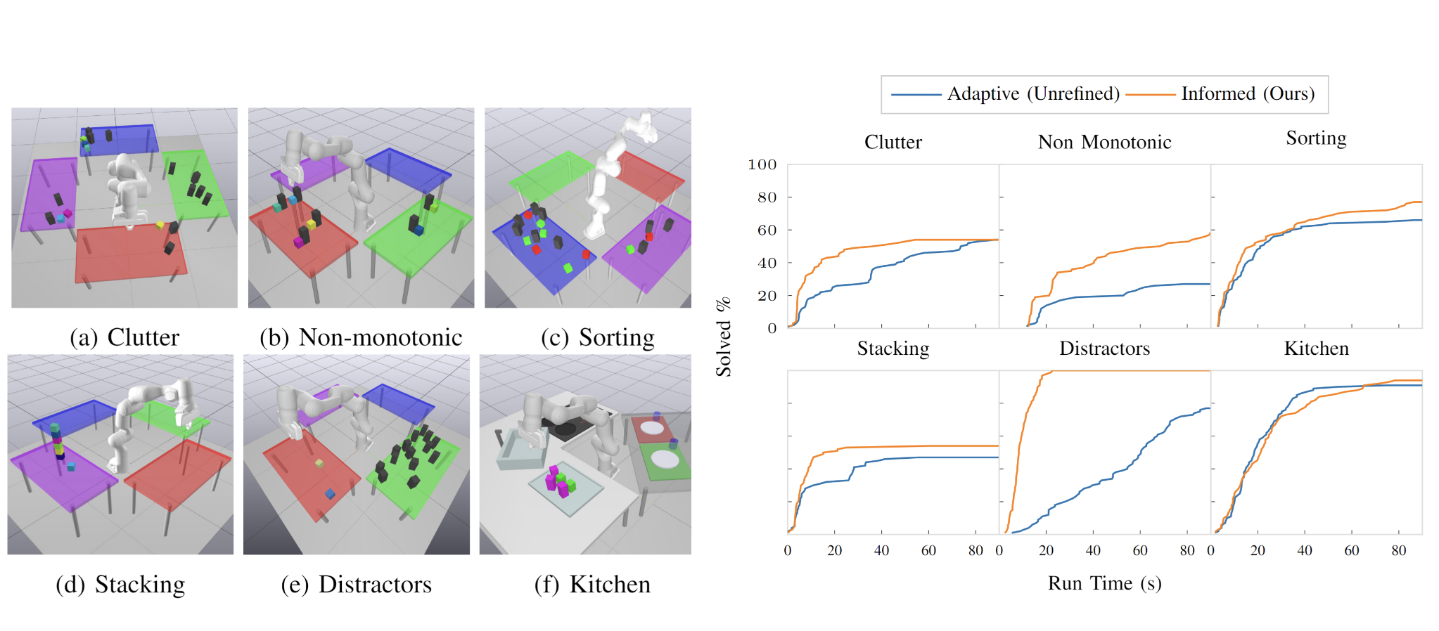
Learning to Rank Objects and Operations from Past Experience
![]()
Learning to Rank Objects and Operations from Past Experience
![]()
Today’s agenda
• Learning programs based on execution traces (NPI - Neural Programmer Interpreters)
• Extending NPI for video-based robot imitation (NTP - Neural Task Programming)
• Inferring sub-task boundaries (TACO - Temporal Alignment for Control)
• Learning to search in Task and Motion Planning (TAMP)
• Generalization through imitation – using hierarchical policies
source: https://www.youtube.com/watch?v=hlvRmLlYHZ0&t=111s&ab_channel=RoboticsScienceandSystems