CSC2626 Imitation Learning for Robotics
Week 5: Learning Reward Functions
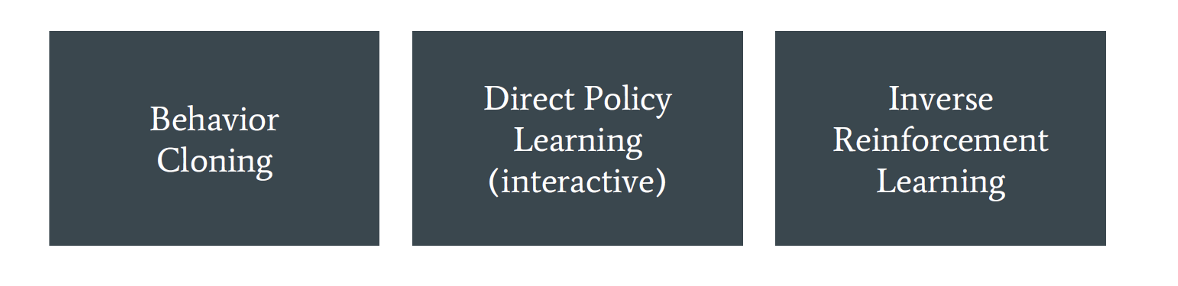
Imitation Learning approaches
• In Imitation Learning, we want to learn to predict the behavior an expert agent would choose.
• So far, we have seen two main paradigms to tackle this problem

Imitation Learning approaches
• In Imitation Learning, we want to learn to predict the behavior an expert agent would choose.
• Today, we introduce a third paradigm: Inverse Reinforcement Learning (IRL)
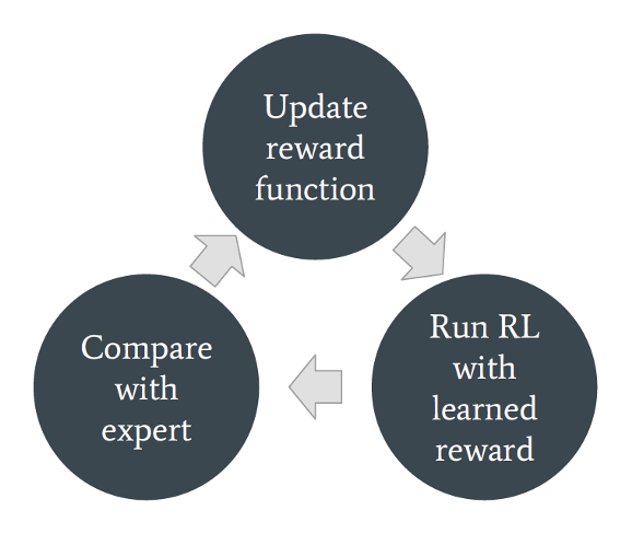
Basic Principle
- IRL reduces the imitation problem to:
- Recovering a reward function given a set of demonstrations.
- Solving the MDP using RL to recover the policy, conditioned on our learned reward.
- IRL assumes that the reward function provides the most concise and transferable definition of the task
Maximum Entropy Principle [Ziebart et al. 2008]
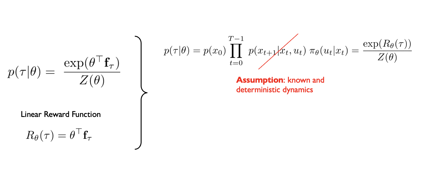
Maximum Entropy IRL [Ziebart et al. 2008]
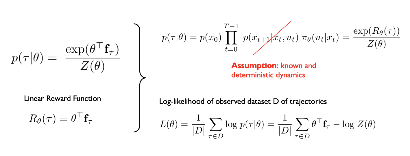
Maximum Entropy IRL [Ziebart et al. 2008]
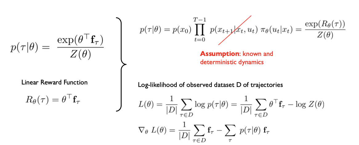
Maximum Entropy IRL [Ziebart et al. 2008]
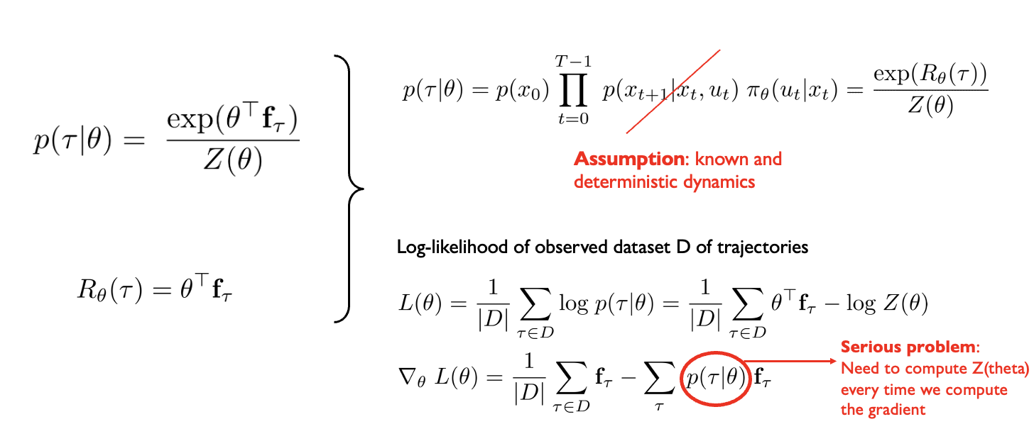
Maximum Entropy IRL [Ziebart et al. 2008]
State visitation distribution
The exponential growth of paths with the MDPs time horizon makes enumeration-based approaches infeasible.
The authors proposed a DP algorithm similar to value iteration to compute the state visitation distribution efficiently.
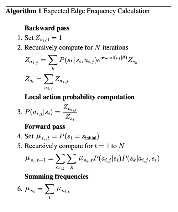
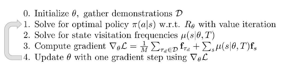
MaxEnt high-level algorithm
Application: Driver Route Modelling
- Maximize the probability of demonstrated paths using MaxEnt IRL*
- Baselines:
- Time-based: Based on expected time travels. Weights the cost of a unit distance of road to be inversely proportional to the speed of the road.
- Max-margin [Ratliff et al. 2006]: Model capable of predicting new paths, but incapable of density estimation. Directly measures disagreement between the expert and learned policy
- Action-based [Ramachandran et al. 2007, Neu et al. 2007]: The choice of an action is distributed according to the future expected reward of the best policy after taking that action. Suffers from label bias (local distribution of probability mass):
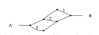
MaxEnt: paths 1, 2, 3 will have 33% probability
Action-based: 50% path 3, 25% paths 1 and 2
*applied to a “fixed class of reasonably good paths” instead of the full training set
Application: Driver Route Modelling
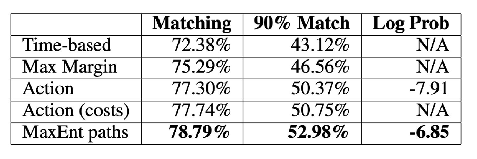
- Matching: Average percentage of distance matching
- 90% Match: Percentage of examples with at least 90% matching distance
- Log Prob: Average log probability
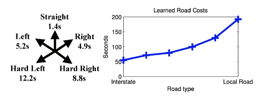
Application: Driver Route Modelling
- Learned costs:
- Additionally, learned a fixed per edge cost of 1.4 seconds to penalize roads composed of many short paths
Application: Driver Route Modelling
- Predicting destination: so far we have only described situations where the driver intended destination is known. We can use Bayes rule to predict destination* given our current model.
\[ P(\text{dest} \mid \tilde{\tau}_{A \rightarrow B}) \propto P(\tilde{\tau}_{A \rightarrow B} \mid \text{dest}) \, P(\text{dest}) \]
\[ \propto \frac{\sum_{\tau_{B \rightarrow \text{dest}}} e^{\theta^{\top} f_{\tau}}}{\sum_{\tau_{A \rightarrow \text{dest}}} e^{\theta^{\top} f_{\tau}}} \, P(\text{dest}) \]
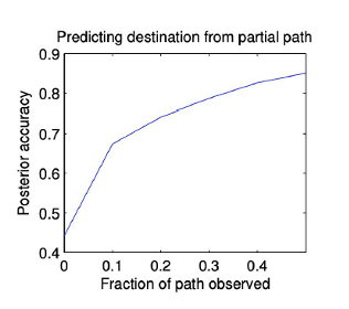
*posed as a multiclass classification problem over 5 possible destinations
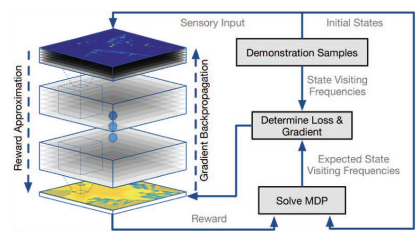
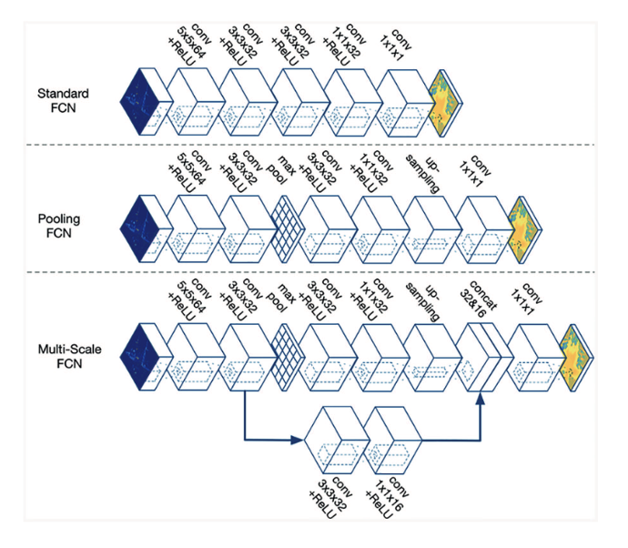
Deep Maximum Entropy IRL [Wulfmeier et al. 2017]
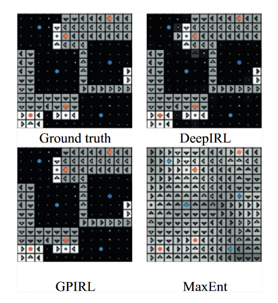
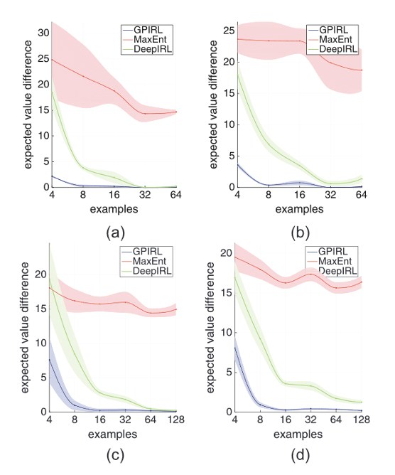
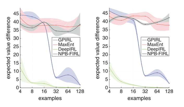
Benchmarking
• Two hidden layers
• ReLU activation
• 1x1 filter weights
• Evaluation metric: expected value difference
• Compared against Linear MaxEnt, GPIRL, NPB-FIRL
Benchmarking
Proposed Network Architectures
Large-scale Demonstration
- 13 drivers
- \(>\) 25,000 trajectories 12m-15m long
- Goal: reward map given features
- Steepness
- Corner cases (underpasses, stairs)
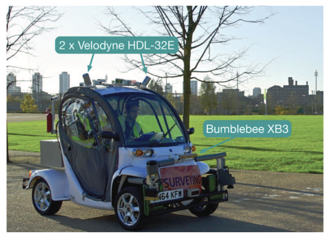
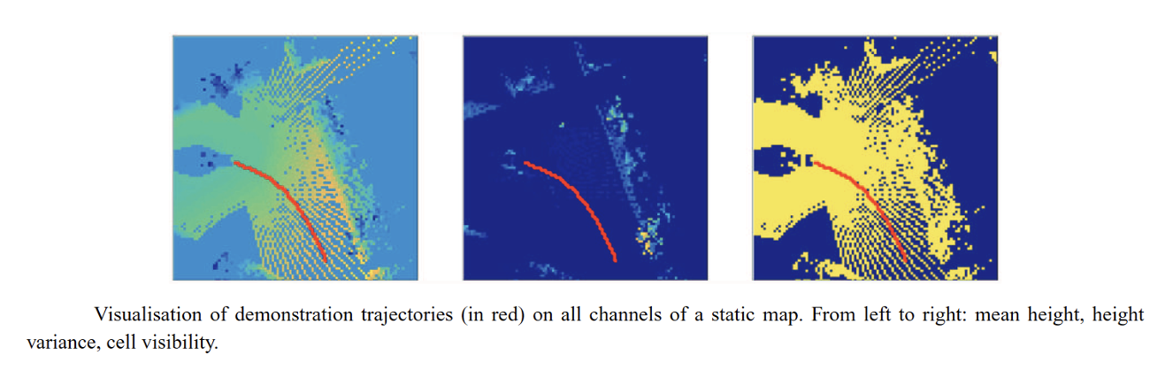
Network Input Data
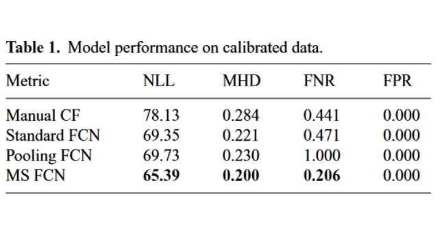
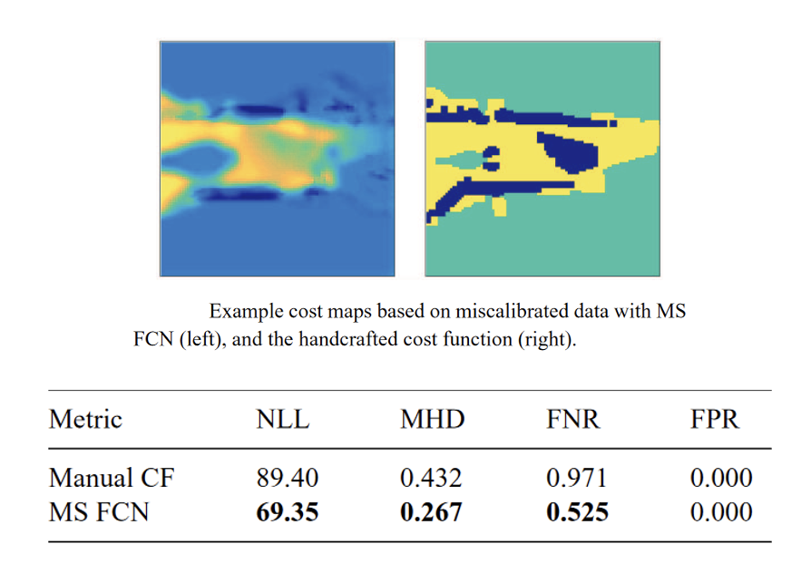
Evaluation
- No absolute ground truth
- Compared against manual cost functions
- Metrics:
- NLL – negative log-likelihood
- MHD – Hausdorff distance
- FNR – False negative rate
- FPR – False positive rate
Robustness to Systematic Noise
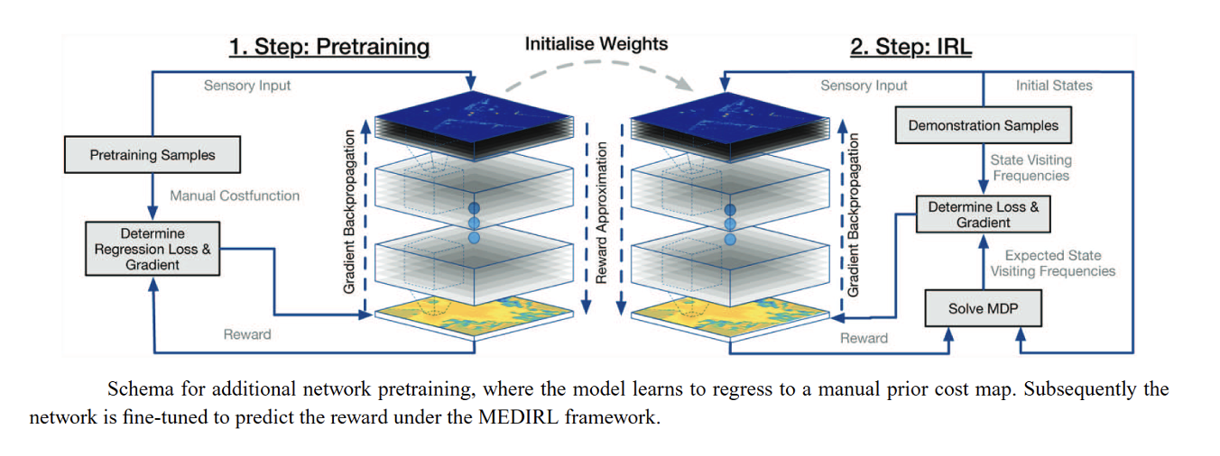
Pretraining
Guided Cost Learning [Finn, Levine, Abbeel et al. 2016]
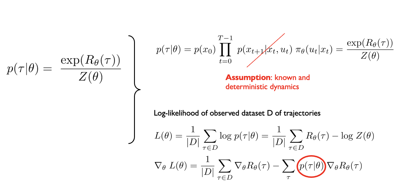
\[ p(\tau|\theta) = \frac{\exp(-c_{\theta}(\tau))}{Z(\theta)} \]
Nonlinear Reward Function
Learned Features
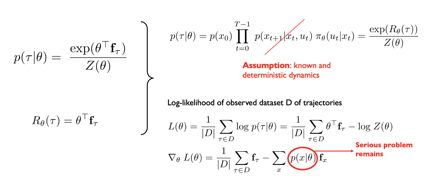
\(p(\tau|\theta) = p(x_0) \prod_{t=0}^{T-1} \underbrace{p(x_{t+1}|x_t, u_t)} \pi_{\theta}(u_t|x_t) = \frac{\exp(-c_{\theta}(\tau))}{Z(\theta)}\)
True and stochastic dynamics (unknown)
Log-likelihood of observed dataset D of trajectories
\[ L(\theta) = \frac{1}{|D|} \sum_{\tau \in D} \log p(\tau|\theta) = \frac{1}{|D|} \sum_{\tau \in D} -c_{\theta}(\tau) - \log Z(\theta) \]
Approximating the gradient of the log-likelihood
\[ p(\tau|\theta) = \frac{\exp(-c_{\theta}(\tau))}{Z(\theta)} \]
Nonlinear Reward Function
Learned Features
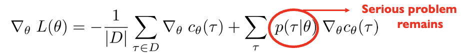
\[ \nabla_{\theta} L(\theta) = -\frac{1}{|D|} \sum_{\tau \in D} \nabla_{\theta} c_{\theta}(\tau) + \underbrace{\sum_{\tau} p(\tau \mid \theta) \nabla_{\theta} c_{\theta}(\tau)} \]
How do you approximate this expectation?
Idea #1: sample from \(p(\tau | \theta)\)
(can you do this)
Approximating the gradient of the log-likelihood
\[ p(\tau|\theta) = \frac{\exp(-c_{\theta}(\tau))}{Z(\theta)} \]
Nonlinear Reward Function
Learned Features
\[ \nabla_{\theta} L(\theta) = -\frac{1}{|D|} \sum_{\tau \in D} \nabla_{\theta} c_{\theta}(\tau) + \underbrace{\sum_{\tau} p(\tau \mid \theta) \nabla_{\theta} c_{\theta}(\tau)} \]
How do you approximate this expectation?
Idea #1: sample from \(p(\tau | \theta)\)
(don’t know the dynamics)
Idea #2: sample from an easier distribution \(q(\tau | \theta)\)
that approximates \(p(\tau | \theta)\)
Importance Sampling
see Relative Entropy Inverse RL by Boularias, Kober, Peters
Importance Sampling
How to estimate properties/statistics of one distribution (p) given samples from another distribution (q)
\[ \begin{align} \mathbb{E}_{x \sim p(x)}[f(x)] &= \int f(x)p(x)\,dx \\ &= \int \frac{q(x)}{q(x)} f(x)p(x)\,dx \\ &= \int f(x)p(x)\frac{q(x)}{q(x)}\,dx \\ &= \mathbb{E}_{x\sim q(x)}\left[ f(x)\frac{p(x)}{q(x)}\right] \\ &= \mathbb{E}_{x\sim q(x)}[f(x)w(x)] \end{align} \]
Weights = likelihood ratio, i.e. how to reweigh samples to obtain statistics of p from samples of q
Importance Sampling: Pitfalls and Drawbacks
What can go wrong?
\[ \begin{align} \mathbb{E}_{x \sim p(x)}[f(x)] &= \int f(x)p(x)\,dx \\ &= \int \frac{q(x)}{q(x)} f(x)p(x)\,dx \\ &= \int f(x)p(x)\frac{q(x)}{q(x)}\,dx \\ &= \mathbb{E}_{x\sim q(x)}\left[ f(x)\frac{p(x)}{q(x)}\right] \\ &= \mathbb{E}_{x\sim q(x)}[f(x)w(x)] \end{align} \]
Problem #1:
If q(x) = 0 but f(x)p(x) > 0
for x in non-measure-zero
set then there is estimation bias
Problem #2:
Weights measure mismatch between q(x) and p(x). If mismatch is large then some weights will dominate. If x lives in high dimensions a single weight may dominate
Problem #3:
Variance of estimator is high if (q – fp)(x) is high
For more info see:
#1, #3: Monte Carlo theory, methods, and examples, Art Owen, chapter 9
#2: Bayesian reasoning and machine learning, David Barber, chapter 27.6 on importance sampling
Importance Sampling
What is the best approximating distribution q?
\[ \begin{align} \mathbb{E}_{x \sim p(x)}[f(x)] &= \int f(x)p(x)\,dx \\ &= \int \frac{q(x)}{q(x)} f(x)p(x)\,dx \\ &= \int f(x)p(x)\frac{q(x)}{q(x)}\,dx \\ &= \mathbb{E}_{x\sim q(x)}\left[ f(x)\frac{p(x)}{q(x)}\right] \\ &= \mathbb{E}_{x\sim q(x)}[f(x)w(x)] \end{align} \]
Best approximation \(q(x) \propto f(x)p(x)\)
Importance Sampling
How does this connect back to partition function estimation?
\[ \begin{align} Z(\theta) &= \sum_{\tau} \exp(-c_{\theta}(\tau)) \\ &= \sum_{\tau} \exp(-c_{\theta}(\tau)) \\ &= \sum_{\tau} \frac{q(\tau|\theta)}{q(\tau|\theta)} \exp(-c_{\theta}(\tau)) \\ &= \mathbb{E}_{\tau \sim q(\tau|\theta)} \left[ \frac{\exp(-c_{\theta}(\tau))}{q(\tau|\theta)} \right] \end{align} \]
Best approximation \(q(\tau | \theta) \propto exp(-c_{\theta} (\tau))\)
Cost function estimate changes at each gradient step
Therefore the best approximating distribution should change as well
Approximating the gradient of the log-likelihood
\[ p(\tau|\theta) = \frac{\exp(-c_{\theta}(\tau))}{Z(\theta)} \]
Nonlinear Reward Function
Learned Features
\[ \nabla_{\theta} L(\theta) = -\frac{1}{|D|} \sum_{\tau \in D} \nabla_{\theta} c_{\theta}(\tau) + \underbrace{\sum_{\tau} p(\tau \mid \theta) \nabla_{\theta} c_{\theta}(\tau)} \]
How do you approximate this expectation?
Idea #1: sample from \(p(\tau | \theta)\)
(don’t know the dynamics)
Idea #2: sample from an easier distribution \(q(\tau | \theta)\)
that approximates \(p(\tau | \theta)\)


Recall from Guided Policy Search
\(\underset{q(\tau)}{\text{argmin}} \quad \mathbb{E}_{\tau \sim q(\tau)}[c(\tau)]\)
\(\text{subject to} \quad q(x_{t+1}|x_t, u_t) = \mathcal{N}(x_{t+1}; f_{xt}x_t + f_{ut}u_t, F_t) \qquad \color{red}\Leftarrow \quad \text{Learn linear Gaussian dynamics}\)
\(\qquad \qquad \text{KL}(q(\tau) || q_{\text{prev}}(\tau)) \leq \epsilon\)

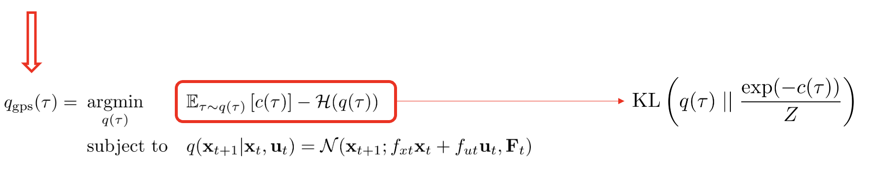
\(q_{\text{gps}}(\tau) = \underset{q(\tau)}{\text{argmin}} \quad \mathbb{E}_{\tau \sim q(\tau)}[c(\tau)] - \mathcal{H}(q(\tau))\)
\(\qquad \qquad \text{subject to} \quad q(x_{t+1}|x_t, u_t) = \mathcal{N}(x_{t+1}; f_{xt}x_t + f_{ut}u_t, F_t)\)
\(q_{\text{gps}}(\tau) = q(x_0) \prod_{t=0}^{T-1} q(x_{t+1}|x_t, u_t)q(u_t|x_t)\)
\(\qquad \color{red} \uparrow \qquad \quad \uparrow\)
Linear Gaussian
dynamics and controller
Run controller on the robot
Collect trajectories
\(q_{prev} = q_{gps}\)
Recall from Guided Policy Search
\(\arg\min_{q(\tau)} \; \mathbb{E}_{\tau \sim q(\tau)} [c(\tau)]\)
\(\begin{align} \text{subject to} & \quad q(x_{t+1} \mid x_t, u_t) = \mathcal{N}(x_{t+1}; f_{xt}x_t + f_{ut}u_t, F_t) \color{red} \qquad \Leftarrow \text{Learn Linear Gaussian dynamics} \\ & \text{KL}(q(\tau) \parallel q_{\text{prev}}(\tau)) \leq \epsilon \end{align}\)
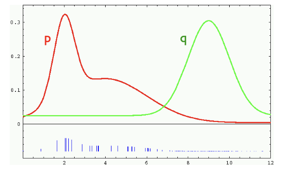
Given a fixed cost function c, the linear
Gaussian controllers that GPS computes
induce a distribution of trajectories close to
\(\frac{\exp(-c(\tau))}{Z}\)
i.e. good for importance sampling of the partition function Z
Guided Cost Learning [rough sketch]
Collect demonstration trajectories D
Initialize cost parameters \(\theta_0\)
![]()
Do forward optimization using Guided Policy Search for cost function \(c_{\theta_t} (\tau)\)
and compute linear Gaussian distribution of trajectories \(q_{gps} (\tau)\)
\(\nabla_{\theta} L(\theta) = -\frac{1}{|D|} \sum_{\tau \in D} \nabla_{\theta} c_{\theta}(\tau) + \underbrace{\sum_{\tau} p(\tau \mid \theta) \nabla_{\theta} c_{\theta}(\tau)}\)
Importance sample trajectories from \(q_{gps} (\tau)\)
\(\theta_{t+1} = \theta_t + \gamma \nabla_{\theta} L(\theta_t)\)
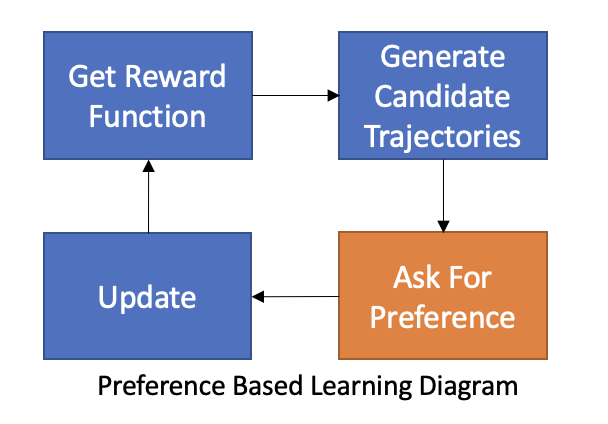
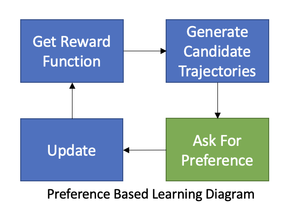
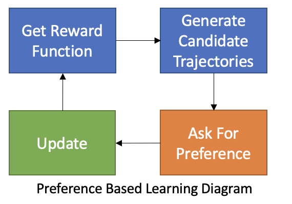
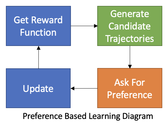
Preference Based Learning
Learn rewards from expert preference
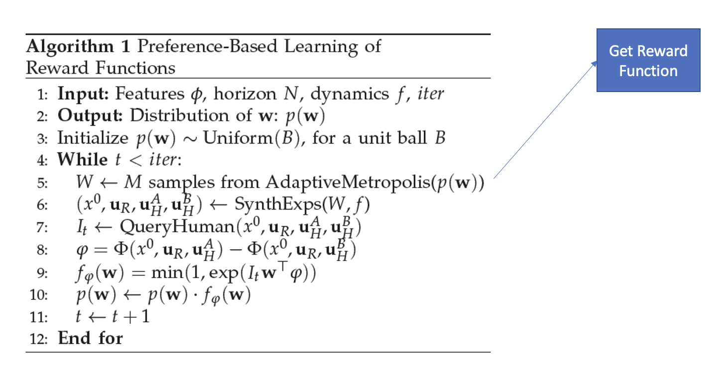
Have an estimate of reward function
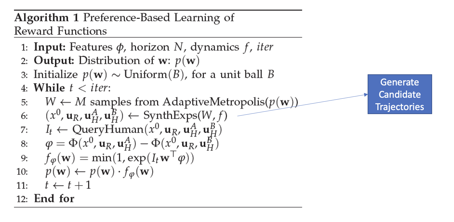
Pick two candidate trajectories
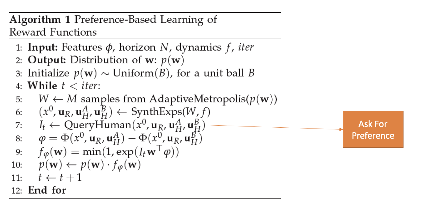
Ask the human which trajectory is preferred
Use preference as feedback to update reward function
• Rewards updated directly
• No inner RL loop
• No probability estimation required
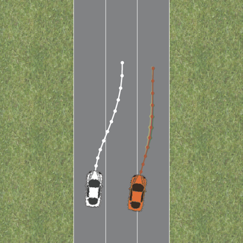
Problem Statement: Autonomous Driving
- 2 vehicles on the road:
- Our orange vehicle denoted 𝐻
- Other white vehicle/robot denoted 𝑅
- States: \((x_H, x_R)\)
- Inputs: \((u_H, u_R)\)
- Dynamics: \(x^{t+1} = f_{HR}(x^t, u_H, u_R)\)
- Finite Trajectories: \(\xi = \{(x^0, u^0_H, u^0_R), \ldots, (x^N, u^N_H, u^N_R)\}\)
- Feasible Trajectories: \(\xi \in \Xi\)
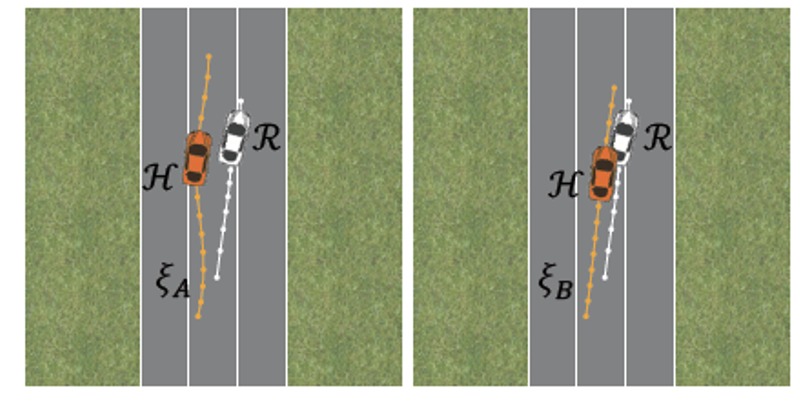
Preference
Given 2 trajectories \(\xi_A\) and \(\xi_B\)
Preference variable 𝐼
\[ I = \begin{cases} +1, & \text{if } \xi_A \text{ is preferred} \\ -1, & \text{if } \xi_B \text{ is preferred} \end{cases} \\ \]
\(\xi_A \text{ or } \xi_B \rightarrow I\)
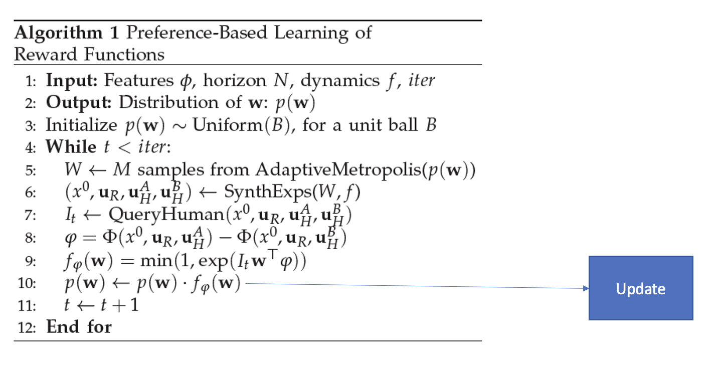
Weight Update
- Assume probabilistic model: weights come from a distribution
- Preference is noisy:
\[ P(I|w) = \begin{cases} \frac{\exp(R_H(\xi_A))}{\exp(R_H(\xi_A)) + \exp(R_H(\xi_B))}, & \text{if } I = +1 \\ \frac{\exp(R_H(\xi_B))}{\exp(R_H(\xi_A)) + \exp(R_H(\xi_B))}, & \text{if } I = -1 \end{cases} \]
- Some simplification:
\(\varphi = \Phi(\xi_A) - \Phi(\xi_B) \qquad \quad f_{\varphi}(w) = P(I|w) = \frac{1}{1 + \exp(-I w^T \varphi)}\)
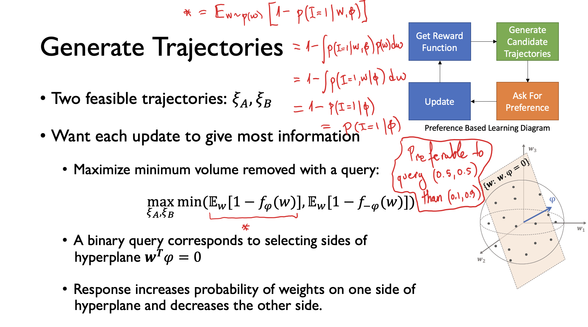
Generate Trajectories
Two feasible trajectories: \(𝜉_𝐴\),\(𝜉_𝐵\)
Want each update to give most information
Maximize minimum volume removed with a query:
\(\underset{{\xi_A, \xi_B}}{\max} \min\left( \mathbb{E}_W[1 - f_{\phi}(w)], \; \mathbb{E}_W[1 - f_{-\phi}(w)] \right)\)
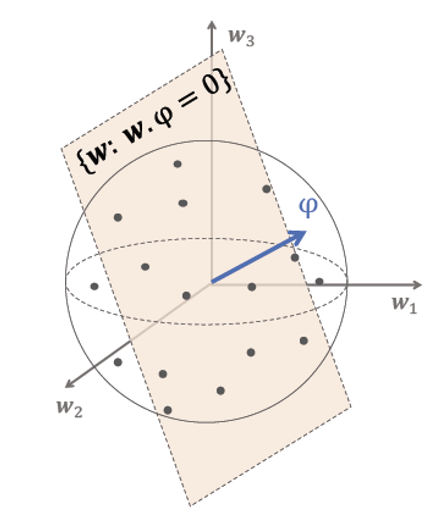
A binary query corresponds to selecting sides of hyperplane \(𝒘^𝑻 𝜑=0\)
Response increases probability of weights on one side of hyperplane and decreases the other side.
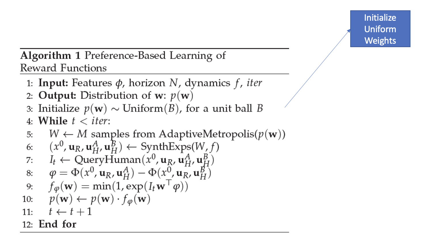
Algorithm Summary
Algorithm Summary
Algorithm Summary
Algorithm Summary
Algorithm Summary
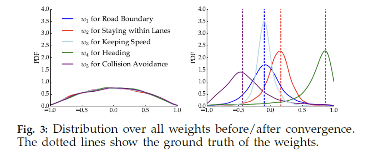
Results
- Weights begin with uniform probability
- Convergence after 200 iterations
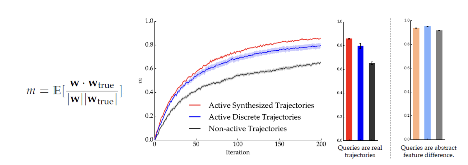
Results
- Rate of convergence, active synthesis is faster!
- Blue curve: generated feasible trajectories not optimized for weight updates
- Black curve: non active trajectories, equivalent to expert dataset
- Lighter colours: training on non feasible trajectories
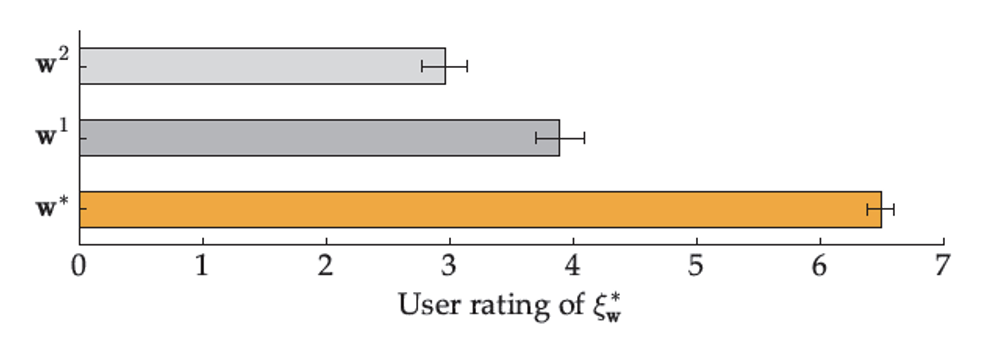
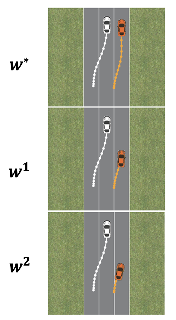
Results
- Perturbation of weights
- Learned weights: \(𝒘^∗\)
- Slightly perturbed weights: \(𝒘^1\)
- Largely perturbed weights: \(𝒘^𝟐\)
- Users prefer \(𝒘^∗\)