where both the policy and the dynamics are stochastic. I.e. we want to learn a globally-valid policy that imitates the actions of locally-valid iLQG policies.
The policy could only control the system from observations \(o\).
The policy \(\pi_\theta(u \mid o_t)\), parametrized by \(\theta\).
At test time, the agent chooses actions according to \(\pi_\theta(u \mid o_t)\) at each time step \(t\), and experiences a loss \(c(x_t \mid o_t) \in [0, 1]\).
The next state is distributed by dynamics \(p(x_{t+1} \mid x_t, u_t)\).
The objective is to learn policy \(\pi_\theta(u \mid o_t)\) such that
One naive way is to train the policy with supervised learning from data generated from an MPC teacher. However, because the state distribution for the teacher and learner are different, the learned policy might fail.
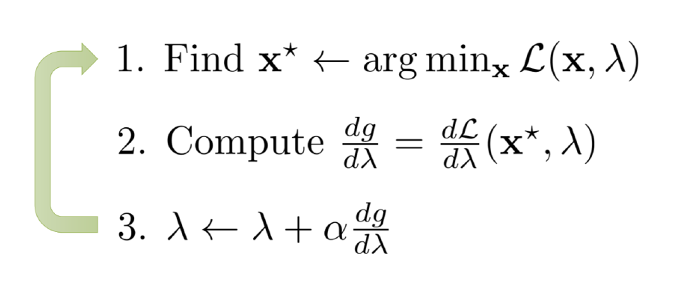
In order to overcome this challenge, an adaptive MPC teacher is used which generates actions from a controller obtained by:
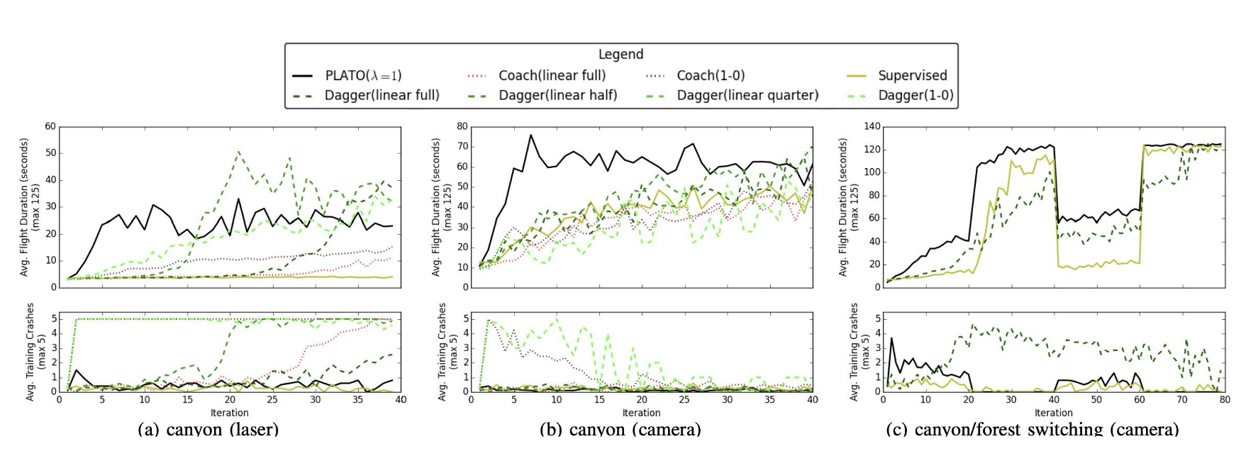
where \(\lambda\) determines the relative importance of matching the learner policy versus optimizing the expected return. Note that the particular MPC algorithm is based on iLQG.
Algorithm
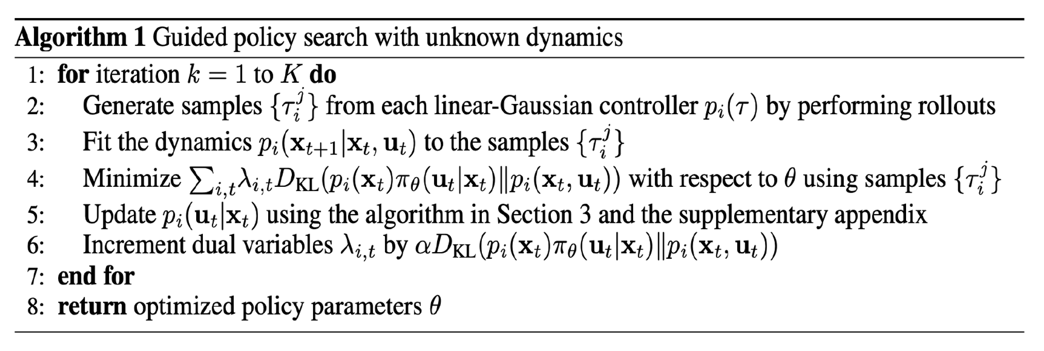
Algorithm 1: PLATO algorithm
Initialize data \(D \leftarrow \emptyset\) for\(i = 1\) to \(N\)do for\(t = 1\) to \(T\)do \(\pi_\lambda^{t}(u_t \mid x_t, \theta) \leftarrow \arg\min_{\pi} J_t(\pi \mid x_t) + \lambda D_{KL}(\pi(u \mid x_t) \,\|\, \pi_{\theta}(u \mid o_t))\)
Sample \(u_t \sim \pi_\lambda^{t}(u \mid x_t, \theta)\) \(\pi^{*}(u_t \mid x_t) \leftarrow \arg\min_{\pi} J(\pi)\)
Sample \(u_t^{*} \sim \pi^{*}(u \mid x_t)\)
Append \((o_t, u_t^{*})\) to dataset \(D\)
State evolves \(x_{t+1} \sim p(x_{t+1} \mid x_t, u_t)\) end for
Train \(\pi_\theta\) on \(D\) end for
Training the learner’s policy
During the supervised learning phase, we minimize the KL-divergence between the learner policy \(\pi_\theta\) and precomputed near-optimal policies \(\pi^*\), which is estimated by iLQG:
Since both \(\pi_\theta\) and \(\pi^*\) are conditionally Gaussian, the KL divergence can be expressed in closed form if we ignore the terms not involving the learner policy means \(\mu_\theta(o_t)\):
In this paper, \(\mu_\theta\) is represented by a NN, and solved by SGD.
Theoretical Analysis
Let \(Q_t(x, \pi, \tilde{\pi})\) denote the cost of executing \(\pi\) for one time step starting from an initial state, and then executing \(\tilde{\pi}\) for the remaining \(t - 1\) time steps. We assume the cost-to-go difference between the learned policy and the optimal policy is bounded: \(Q_t(x, \pi, \pi^*) - Q_t(x, \pi^*, \pi^*) \leq \delta\)
Theorem
Let the cost-to-go \(Q_t(x,\pi,\pi^*) - Q_t(x,\pi^*,\pi^*) \leq \delta\) for all \(t \in \{1,\ldots,T\}\).
Then for PLATO, \(J(\pi_\theta) \leq J(\pi^*) + \delta \sqrt{\epsilon_\theta *} \cdot O(T) + O(1)\)
Therefore, the policy learned by PLATO converges to a policy with bounded cost.
Comparison to DAgger
PLATO could be viewed as a generalization of DAgger, which samples from mixture policy
• RL requires careful reward shaping
• Impractical number of samples to learn (approx. 100 hours)
• Unnatural movement
• Not as robust to environmental variations
• Solution
• Combine RL with demonstrations
• Guide exploration and decrease sample complexity
• Robust and natural looking behaviour
• Demonstration Augmented Policy Gradient (DAPG)
Methodology (Pretraining with BC)
• Exploration in PG achieved with stochastic action distribution
• Poor initialization leads to slow exploration
• Behavioral Cloning (BC) guides exploration
• Reduces sample complexity
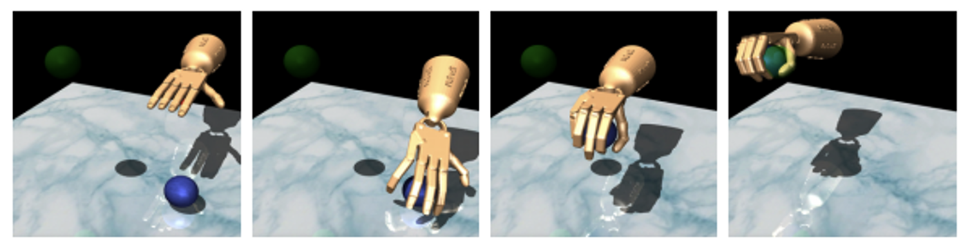
• Mimic actions taken in demonstrations
• Does not guarantee effectiveness of policy due to distributional shift
Methodology (Fine-tuning with augmented loss)
• BC does not make optimal use of demonstrations
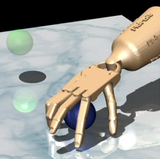
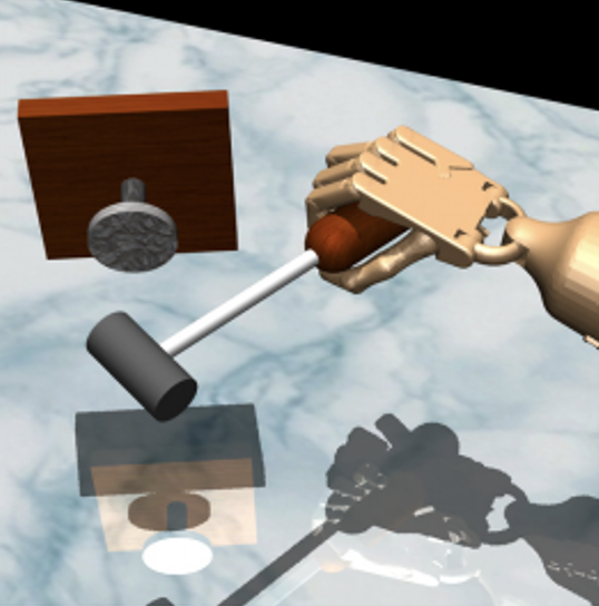
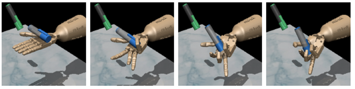
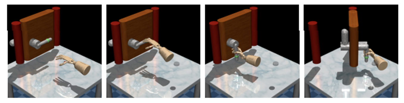
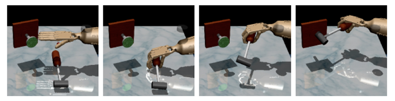
• Cannot learn subtasks (reaching, grasping, hammering)
• BC policy (only grasping)
• Capturing all data
\[
w(s, a) = \lambda_0 \lambda_1^k \max_{(s', a') \in \rho_\pi} A^\pi(s', a') \quad \forall (s, a) \in \rho_D
\]
Policy gradient
Behavioral cloning
\(\uparrow\)
Dataset from policy
\(\uparrow\)
Dataset from
demonstrations
\(\uparrow\)
Weighting
function
\(\downarrow\) iteration
\(\uparrow \quad \uparrow\)
hyperparameters
Results 1
Reinforcement learning from scratch
• Can RL cope with high dimensional manipulation tasks ?
• Is it robust to variations in environment ?
• Are movements safe and can they be used on real hardware ?
• Compare NPG vs DDPG (Deep Deterministic Policy Gradient)
• DDPG is a policy gradient actor-critic algorithm that is off-policy
• Stochastic policy for exploration, estimates deterministic policy
• Score based on percentage of successful trajectories (100 samples)
• Sparse Reward vs Reward shaping
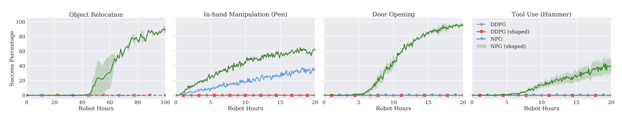
Results 1
Reinforcement learning from scratch
• NPG learns with reward shaping, DDPG fails to learn
• DDPG is sample efficient but sensitive to hyper-parameters
• Resulting policies have unnatural behaviors
• Poor sample efficiency, cant use on hardware
• Cannot generalize to unseen environment (weight and ball size change)
Results 2
Reinforcement learning with demonstrations
• Does incorporating demonstrations reduce learning time?
• Comparison of DAPG vs DDPGfD (.. from Demonstrations)?
• Does it result in human like behaviour ?
• DDPGfD better version of DDPG (demonstrations in replay buffer, prioritized experience replay, n-step returns, regularization)
• Only use sparse rewards
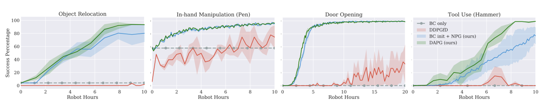
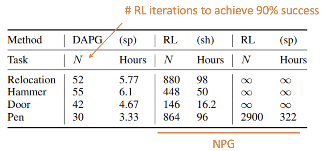
Results 2
Reinforcement learning with demonstrations
• DAPG outperforms DDPGfD
• DAPG requires few robot hours
• Can be used on real hardware
• Robust and human behavior
• Generalizes to unseen environment
Future Work
• Tests on real hardware
• Reduce sample complexity using novelty based exploration methods
• Learn policies from raw visual inputs and tactile sensing
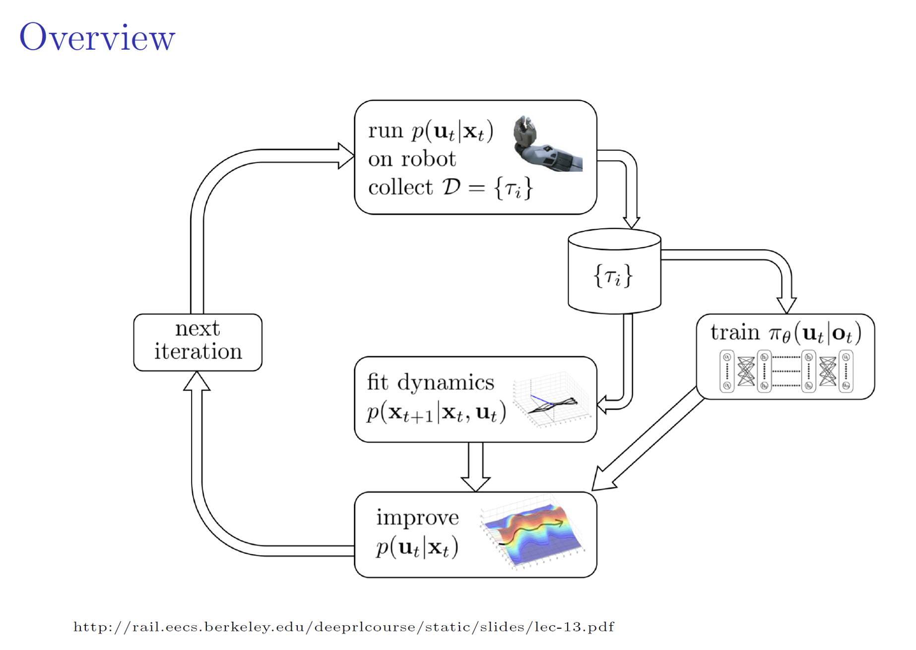
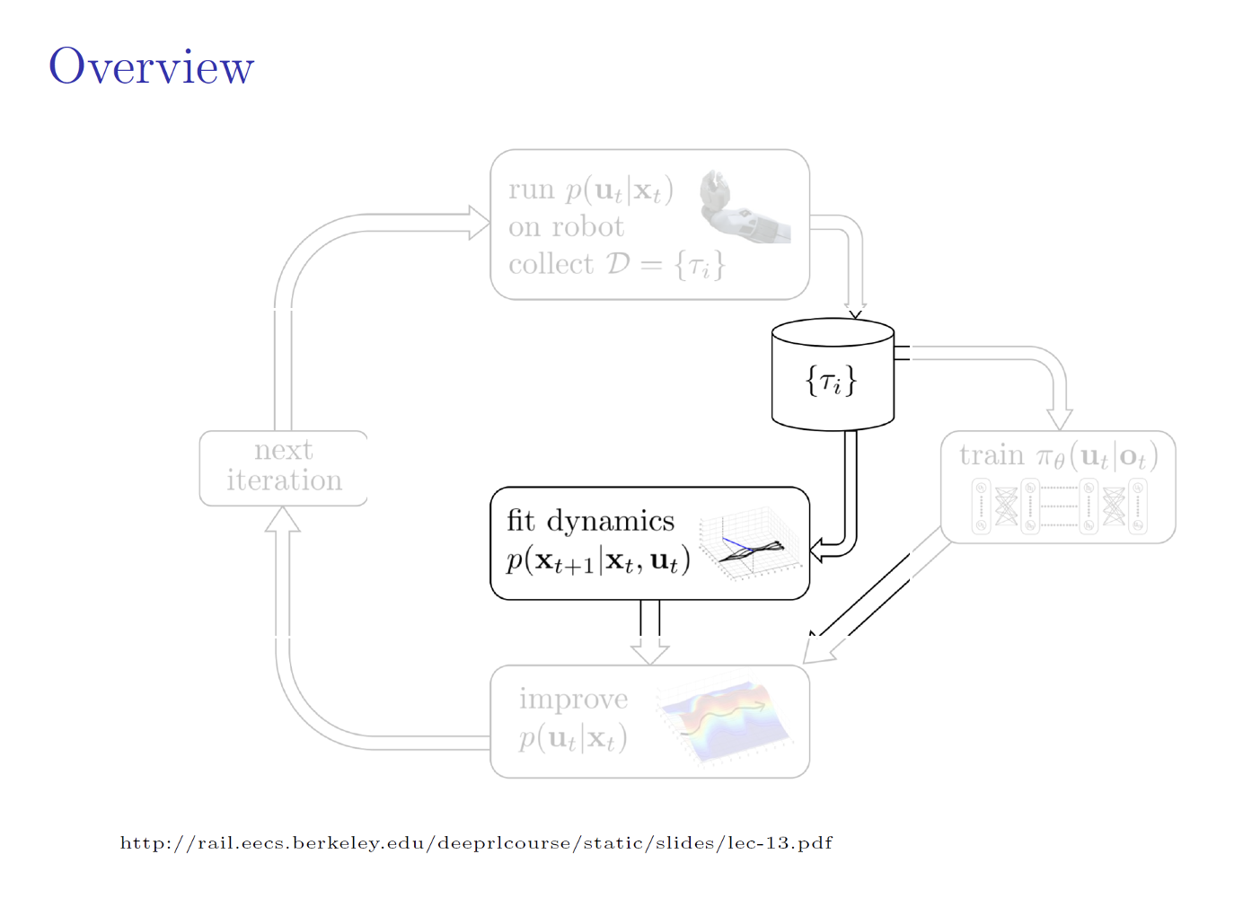
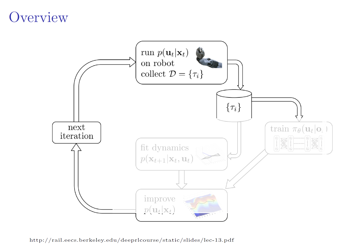
• Policy learning from adaptive MPC with privileged information (PLATO)
• Combining behavioral cloning and RL
• Dynamic movement primitives (DMPs)
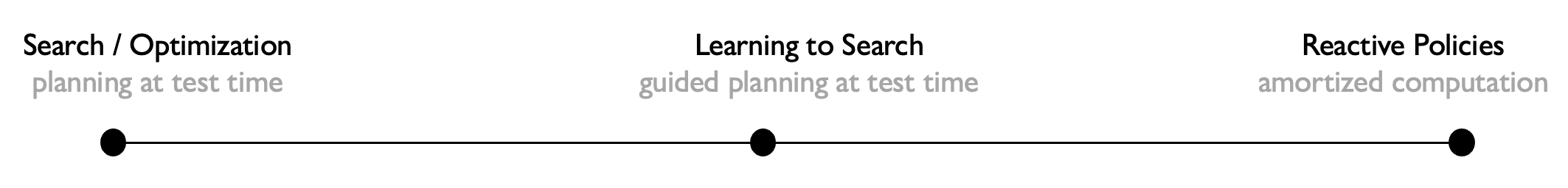
• Expert iteration & learning to search
From Search to Learning and Back
Logic Geometric Programming
Marc Toussaint et al. IJCAI’15, RSS’17
PDDLStream Planners
Caelan Garret et al. ICAPS’20
TAMP = SMT + Motion Planning
Neil Dantam et al. IJRR’18
. . .
\(-\) Need to specify symbols / logic
\(-\) Slow to plan, not very reactive
\(+\) Generalize
\(+\) No training data
Learning to Guide TAMP
Beomjoom Kim et al., AAAI’18
PLOI
Tom Silver, Rohan Chitnis et al. AAAI’21
Deep Visual Heuristics
Danny Driess et al. ICRA’20
Learning to Search for TAMP
Mohamed Khodeir et al. RAL’22, ICRA’23
Text2Motion
Chris Agia et al. ICRA’23
\(-\) Need to specify symbols / logic
\(+\) Can be made fast, reactive
\(+\) Generalize
\(+\) Few training data needed
PaLM-E
Danny Driess et al. ’23
SayCan
Michael Ahn et al. CoRL‘23
RT-1
Anthony Brohan et al. ’22
Deep Affordance Foresight
Danfei Xu et al. ICRA’21
PlaNet, Dreamer, Hierarchical RL
Danijar Hafner et al.
\(+\) Symbols not needed
\(+\) Fast, reactive
\(-\) Do not generalize
\(-\) Large data regime
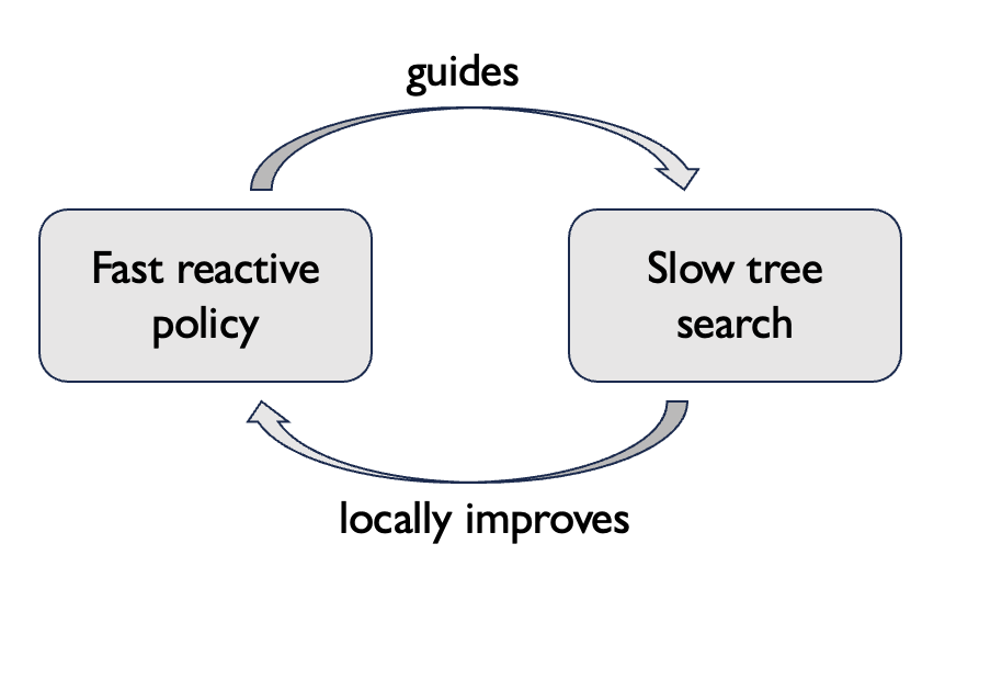
Learning to Plan via Expert Iteration
If we do multiple rounds of heuristic learning and tree search, we could potentially get:
• monotonic improvement guarantees for the policy / planning heuristic
• convergence to a point where tree search and the policy are equally good
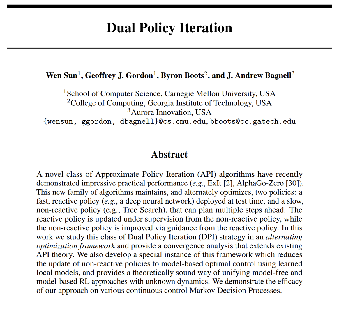
Dual Policy Iteration. Sun, Gordon, Boots, Bagnell. NeurIPS’18.
Thinking Fast and Slow with Deep Learning and Tree Search. Anthony, Tian, Barber. NeurIPS’17.
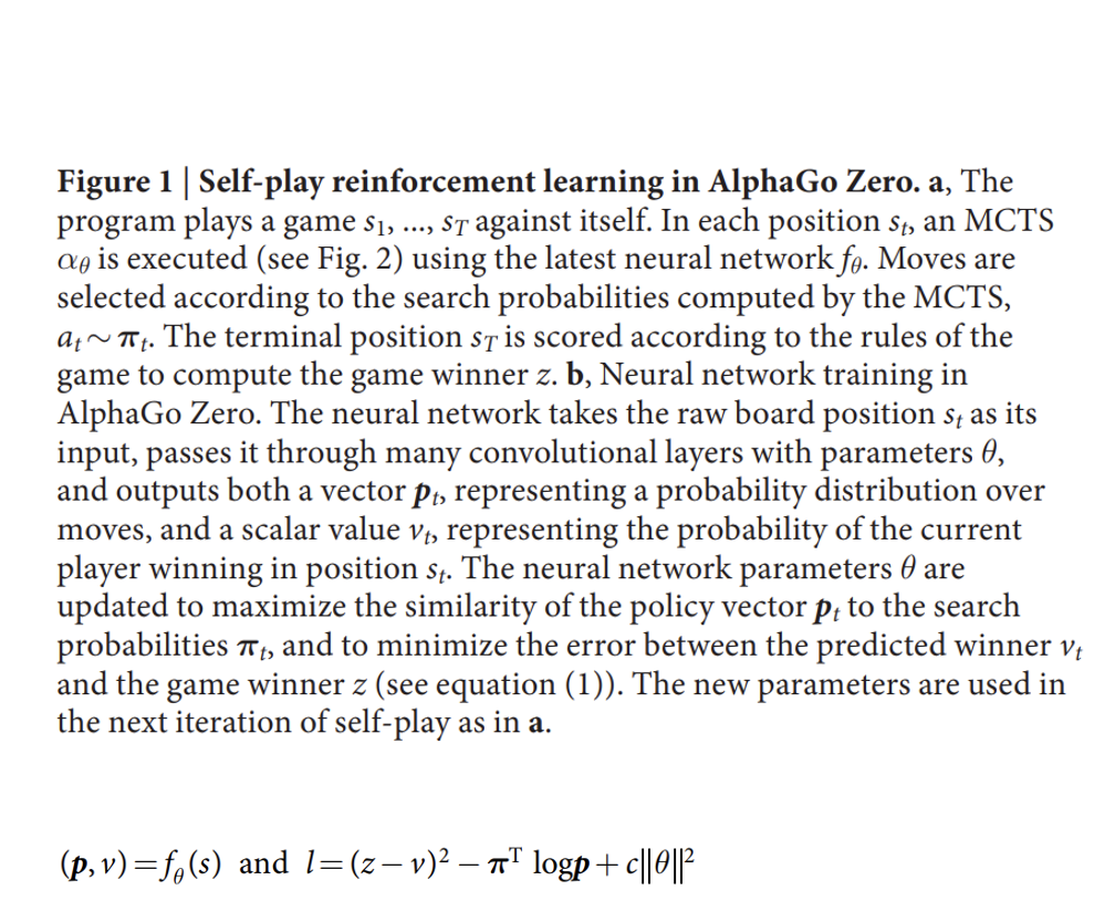
AlphaGo Zero: Mastering the Game of Go Without Human Knowledge. Silver, Schrittwieser, Simonyan, Antonoglou. Nature’17.
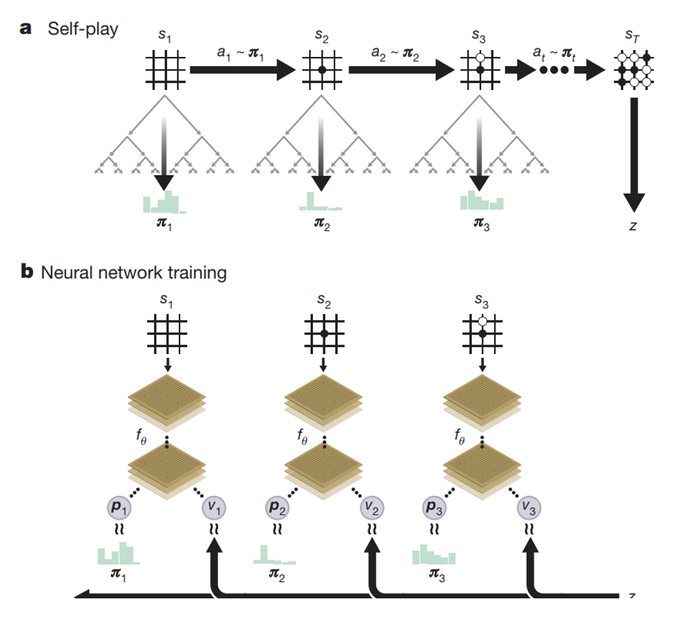
AlphaGo Zero
AlphaGo Zero: Mastering the Game of Go Without Human Knowledge. Silver, Schrittwieser, Simonyan, Antonoglou. Nature’17.
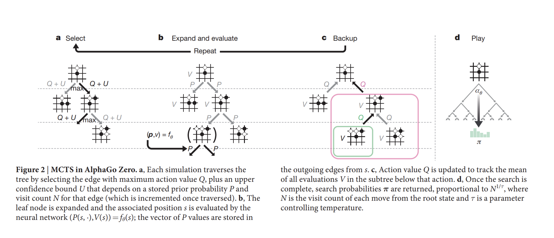
MCTS in AlphaGo Zero
AlphaGo Zero: Mastering the Game of Go Without Human Knowledge. Silver, Schrittwieser, Simonyan, Antonoglou. Nature’17.
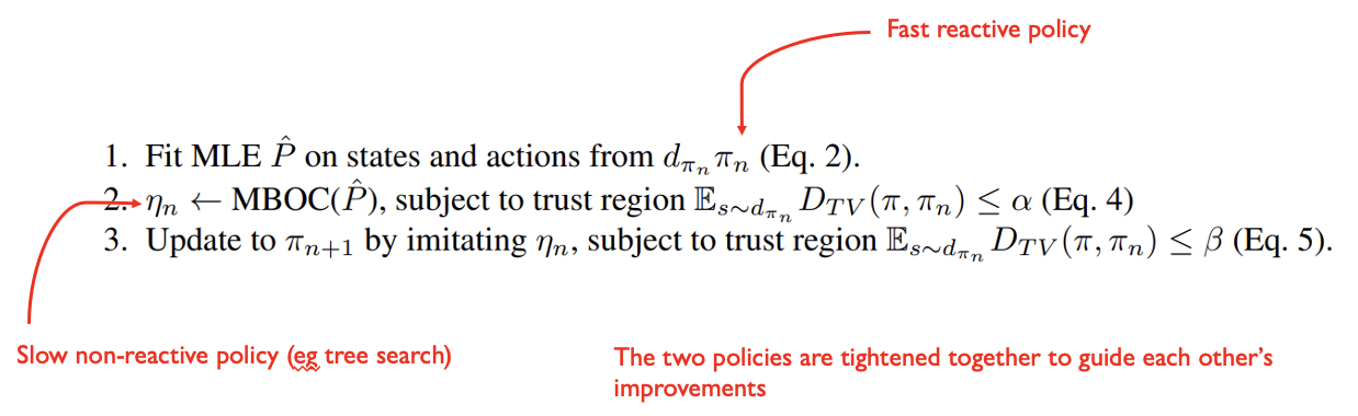
A policy optimization framework that includes
Guided Policy Search
Expert Iteration
AlphaGo Zero
“Thinking fast and slow”
AggreVaTeD (a varianbt of DAgger)
as special cases and provides conditions under which we expect monotonic improvement of the fast, reactive policy.
\[
\begin{array}{ll}
\text{1.} & \text{Fit MLE } \hat{P} \text{ on states and actions from } d_{\pi_n} \pi_n \text{ (Eq. 2).} \\
\text{2.} & \eta_n \leftarrow \text{MBOC}(\hat{P}), \text{ subject to trust region } \mathbb{E}_{s \sim d_{\pi_n}} D_{TV}(\pi, \pi_n) \leq \alpha \text{ (Eq. 4)} \\
\text{3.} & \boxed{\text{Update to } \pi_{n+1} \text{ by imitating } \eta_n, \text{ subject to trust region } \mathbb{E}_{s \sim d_{\pi_{\eta}}} D_{TV}(\pi, \pi_n) \leq \beta \text{ (Eq. 5)}}
\end{array}
\]
Main difference with respect to Guided Policy Search
GPS, including the mirror descent version, phrases the update procedure of the reactive policy as
a behavior cloning procedure, i.e., given an expert policy \(\eta\), we perform \(\min_{\pi} D_{KL}(d_{\mu \mu} \,\|\, d_{\pi \pi})^3\)
Note that our approach to updating \(\pi\) is fundamentally on-policy, i.e., we generate samples from \(\pi\).