Prerequisites
Mandatory:
• Introductory machine learning (e.g. CSC411/ECE521 or equivalent)
• Basic linear algebra + multivariable calculus
• Intro to probability
• Programming skills in Python or C++ (enough to validate your ideas)
If you’re missing any of these this is not the course for you.
You’re welcome to audit.
Recommended:
• Experience training neural networks or other function approximators
• Introductory concepts from reinforcement learning or control (e.g. value function/cost-to-go)
If you’re missing this we can organize tutorials to help you.
Grading
Two assignments: 30%
Course project: 60%
In-class panel discussions: 10%
\(\leftarrow\) Individual submissions
\(\leftarrow\) Individual submissions
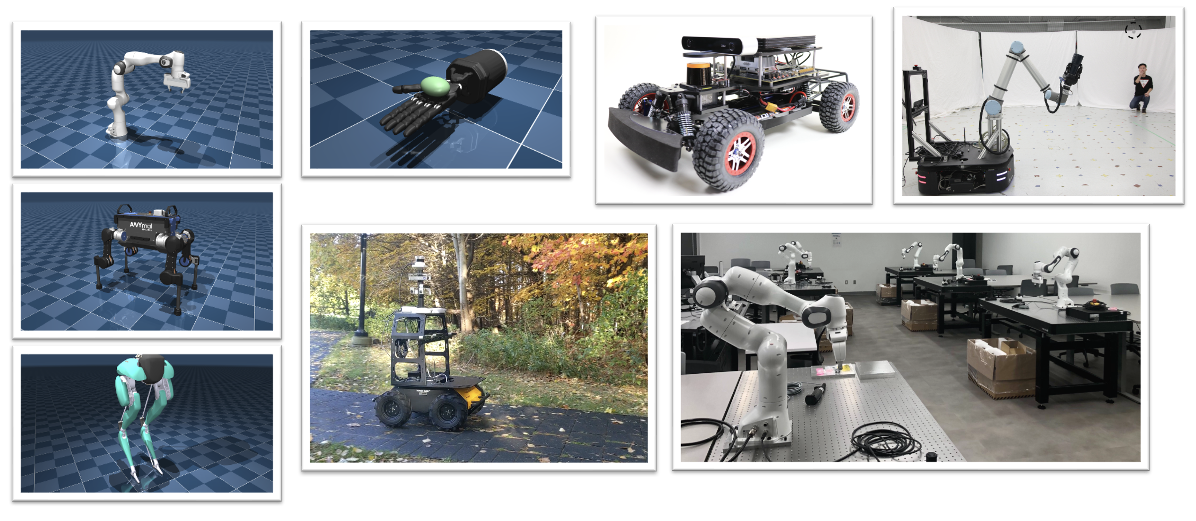
Evaluation environments: simulators & real robots
Guiding principles for this course
Robots do not operate in a vacuum. They do not need to learn everything from scratch.
Humans need to easily interact with robots and share our expertise with them.
Robots need to learn from the behavior and experience of others, not just their own.
Main questions
How can robots incorporate others’ decisions into their own?
How can robots easily understand our objectives from demonstrations?
How do we balance autonomous control and human control in the same system?
\(\quad \color{blue}\Rightarrow\)
Learning from demonstrations Apprenticeship learning Imitation learning
Reward/cost learning Task specification Inverse reinforcement learning Inverse optimal control Inverse optimization
Shared or sliding autonomy
Applications
Any control problem where:
writing down a dense cost function is difficult
there is a hierarchy of decision-making processes
our engineered solutions might not cover all cases
unrestricted exploration during learning is slow or dangerous
Applications
Any control problem where:
writing down a dense cost function is difficult
there is a hierarchy of interacting decision-making processes
our engineered solutions might not cover all cases
unrestricted exploration during learning is slow or dangerous
Applications
Any control problem where:
writing down a dense cost function is difficult
there is a hierarchy of interacting decision-making processes
our engineered solutions might not cover all cases
unrestricted exploration during learning is slow or dangerous
Applications
Any control problem where:
writing down a dense cost function is difficult
there is a hierarchy of interacting decision-making processes
our engineered solutions might not cover all cases
unrestricted exploration during learning is slow or dangerous
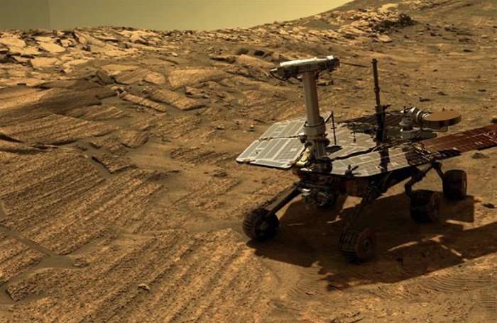
Robot Explorer
Applications
Any control problem where:
writing down a dense cost function is difficult
there is a hierarchy of interacting decision-making processes
our engineered solutions might not cover all cases
unrestricted exploration during learning is slow or dangerous
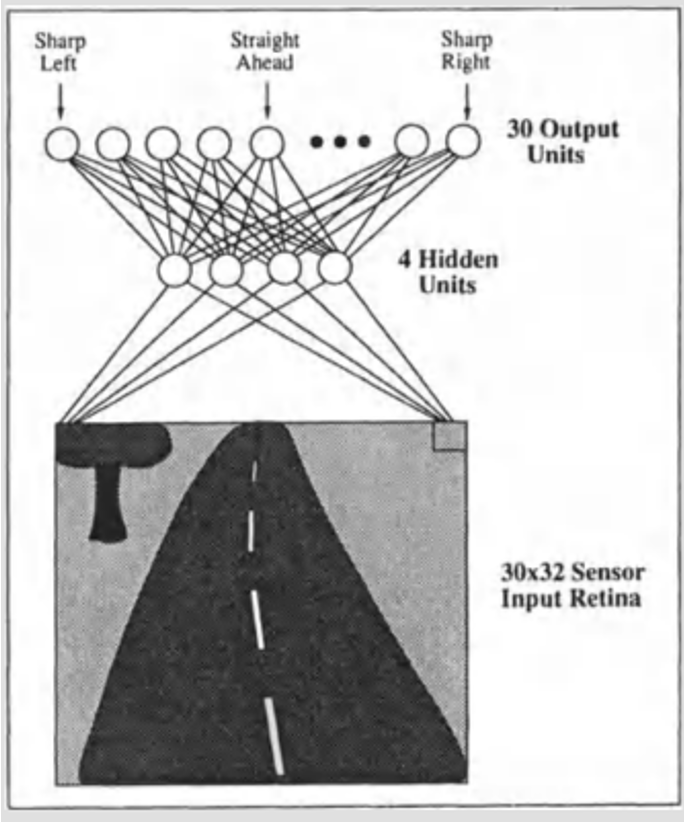
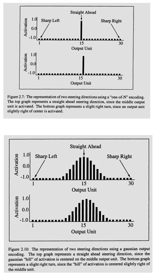
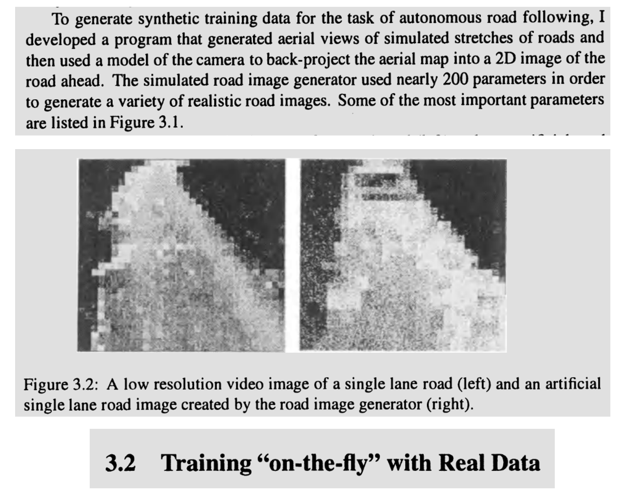
ALVINN: training set
Online updates via backpropagation
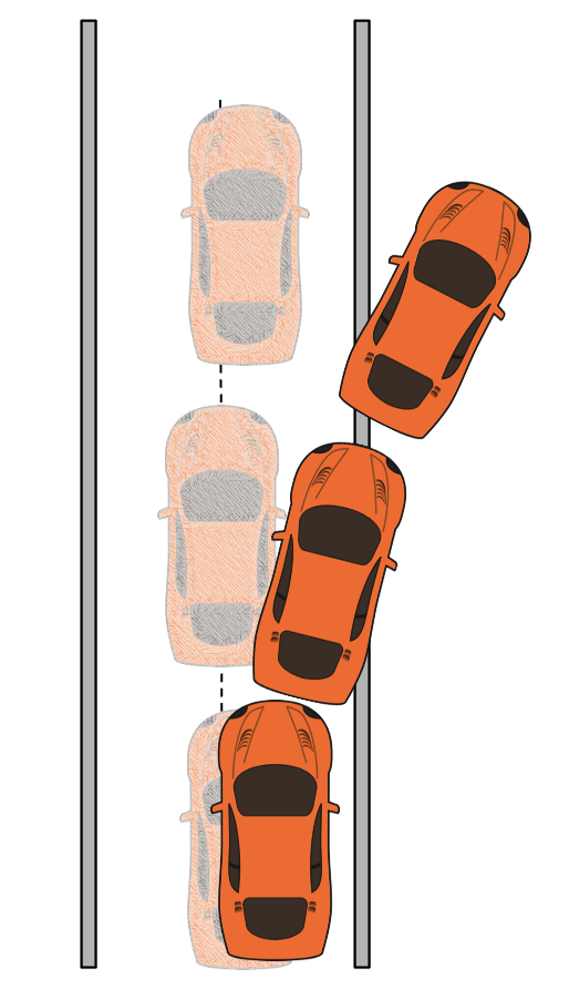
Problems Identified by Pomerleau
Test distribution is different from training distribution (covariate shift)
Catastrophic forgetting
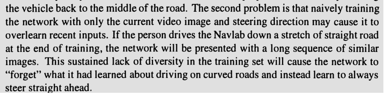
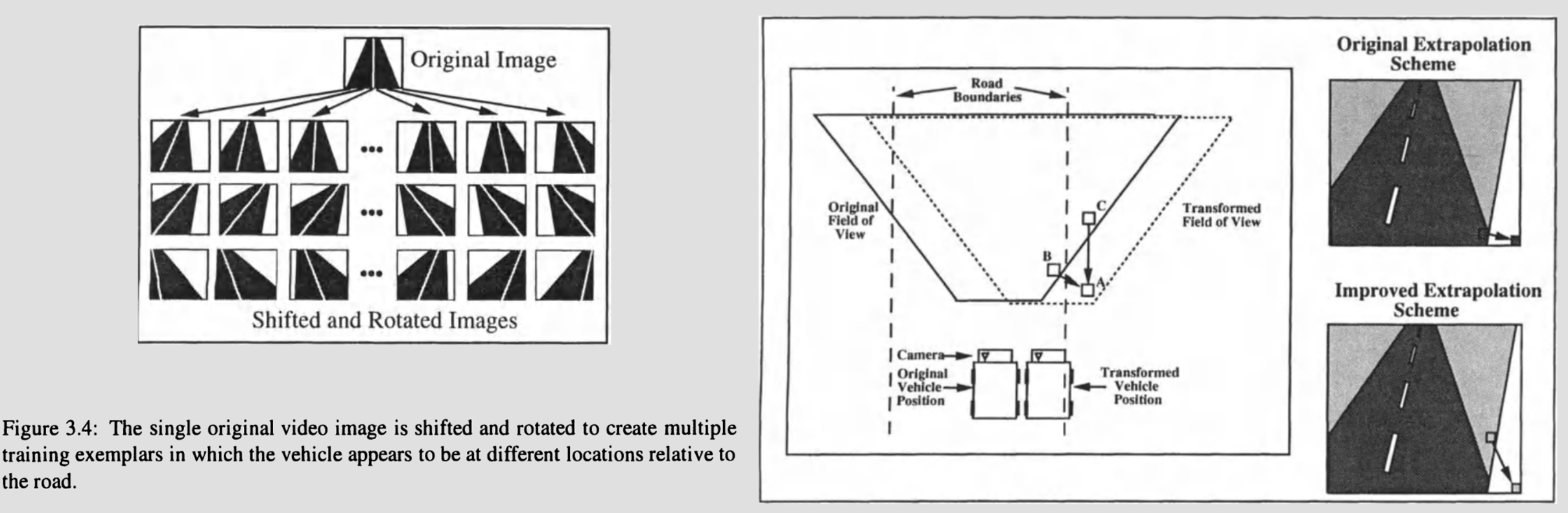
(Partially) Addressing Covariate Shift
(Partially) Addressing Catastrophic Forgetting
Maintains a buffer of old (image, action) pairs
Experiments with different techniques to ensure diversity and avoid outliers
Behavioral Cloning = Supervised Learning
What has changed?
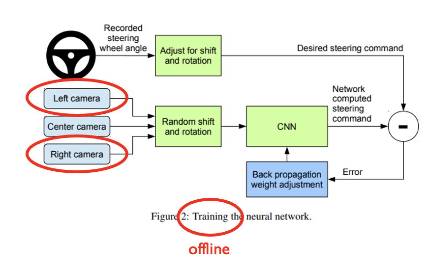
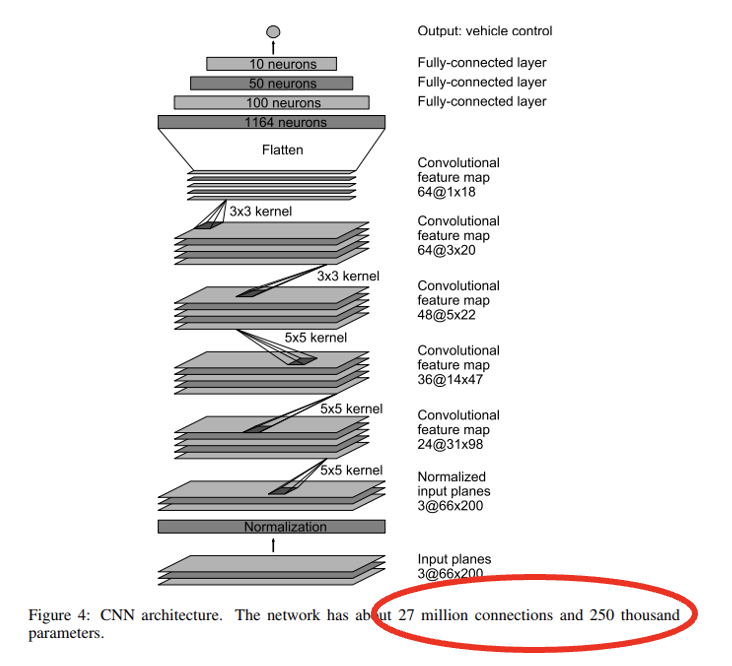
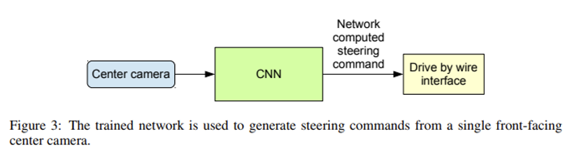
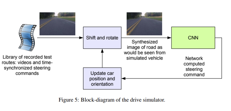
End to End Learning for Self-Driving Cars, Bojarski et al, 2016
What has changed?
“Our collected data is labeled with road type, weather condition, and the driver’s activity (staying in a lane, switching lanes, turning, and so forth).”
End to End Learning for Self-Driving Cars, Bojarski et al, 2016
What has changed?
How much has changed?
VIDEO
How much has changed?
Not a lot for learning lane following with neural networks.
But, there are a few other beautiful ideas that do not involve end-to-end learning.
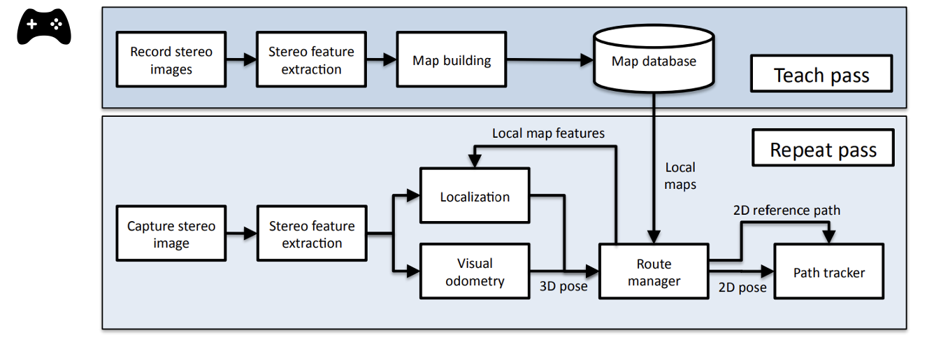
Visual Teach & Repeat
Human Operator or Planning Algorithm
Visual Path Following on a Manifold in Unstructured Three-Dimensional Terrain, Furgale & Barfoot, 2010
Visual Teach & Repeat
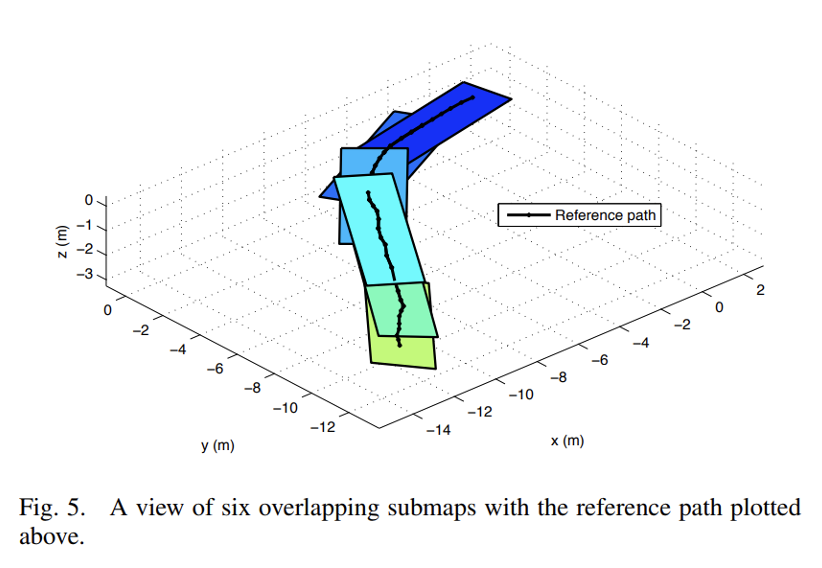
Key Idea #1: Manifold Map
Build local maps relative to the
Key Idea #2: Visual Odometry
Given two consecutive images,
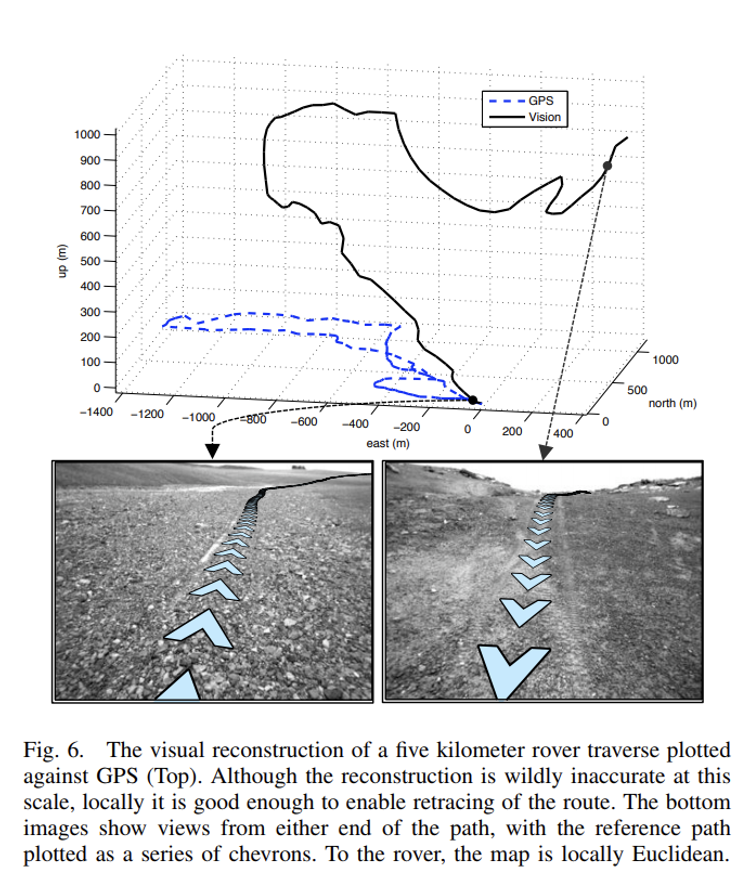
Visual Path Following on a Manifold in Unstructured Three-Dimensional Terrain, Furgale & Barfoot, 2010
Visual Teach & Repeat
Centimeter-level precision in tracking the demonstrated path over kilometers-long trails.
Today’s agenda
• Administrivia
• Topics covered by the course
• Behavioral cloning
• Imitation learning
• Teleoperation interfaces for manipulation
• Imitation via multi-modal generative models (diffusion policy)
• (Time permitting) Query the expert only when policy is uncertain
Nomenclature
• Offline imitation learning:
Learn from a fixed dataset (eg behavioral cloning).
• Online imitation learning:
Learn from a dataset that is not fixed.
Back to Pomerleau
Test distribution is different from training distribution (covariate shift)
(Ross & Bagnell, 2010): How are we sure these errors are not due to overfitting or underfitting?
Maybe the network was too small (underfitting)
Maybe the dataset was too small and the network overfit it
Steering commands \(\pi_\theta (s) = \theta^\top s\) where s are image features
Efficient reductions for imitation learning. Ross & Bagnell, AISTATS 2010.
It was not 1: they showed that even a linear policy can work well.
Imitation learning \(\neq\) Supervised learning
Test distribution is different from training distribution (covariate shift)
(Ross & Bagnell, 2010): IL is a sequential decision-making problem.
• Your actions affect future observations/data.
Imitation Learning \(\qquad \qquad \LARGE \longleftarrow\)
Train/test data are not i.i.d.
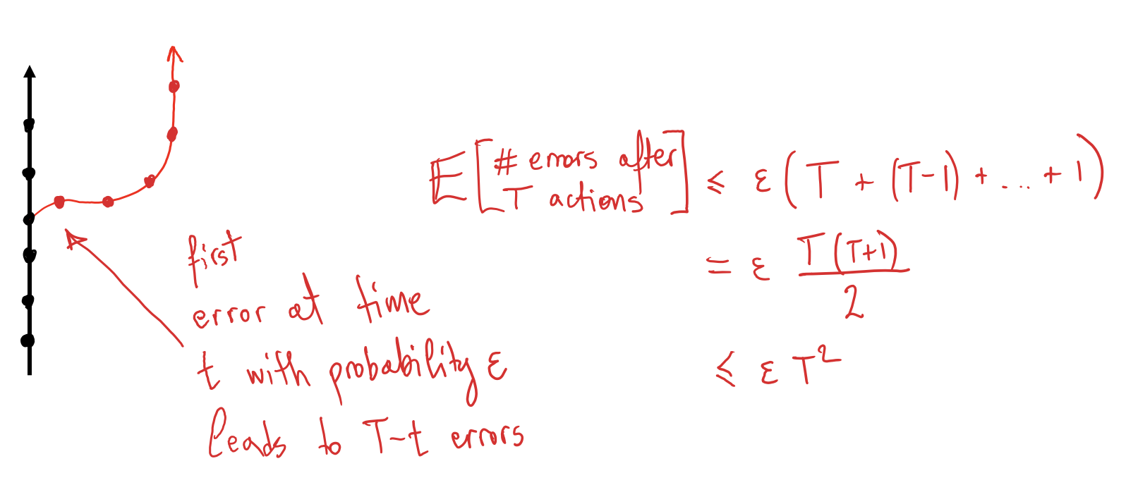
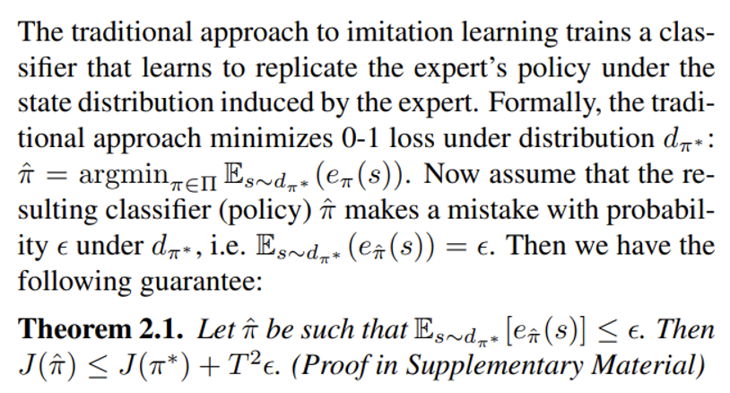
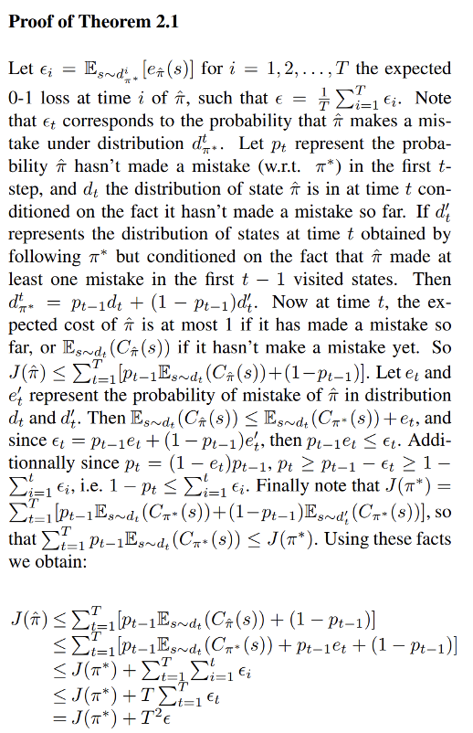
If expected training error \(\delta\) is \(\epsilon\) \[
T^2 \epsilon
\]
Errors compound
Supervised Learning
Assumes train/test data are i.i.d.
If expected training error \(\delta\) is \(\epsilon\) \[
T \epsilon
\]
Errors are independent
Why do errors accumulate quadratically if we use a behavioral cloning policy?
Efficient reductions for imitation learning. Ross & Bagnell, AISTATS 2010.
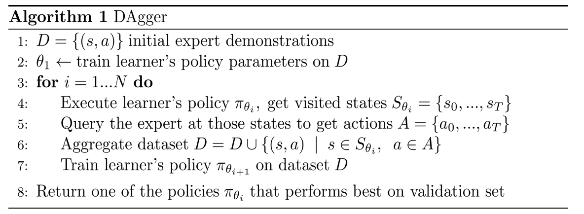
DAgger
(Ross & Gordon & Bagnell, 2011): DAgger, or Dataset Aggregation
• Imitation learning as interactive supervision
• Aggregate training data from expert with test data from execution
A Reduction of Imitation Learning and Structured Prediction to No-Regret Online Learning. Ross, Gordon, Bagnell, AISTATS 2010.
DAgger
(Ross & Gordon & Bagnell, 2011): DAgger, or Dataset Aggregation
• Imitation learning as interactive supervision
• Aggregate training data from expert with test data from execution
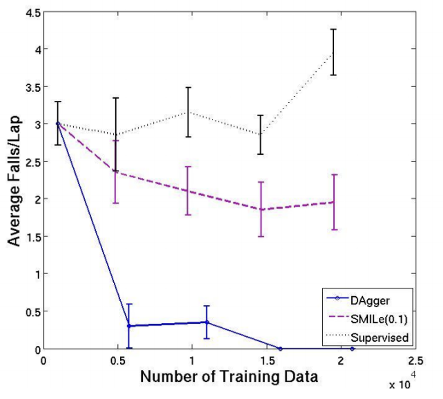
Imitation Learning via DAgger
Train/test data are not i.i.d.
If expected training error on aggr. dataset is \(\epsilon\)
\[
O(T\epsilon)
\]
Errors do not compound
Supervised Learning
Assumes train/test data are i.i.d.
If expected training error is \(\epsilon\)
\[
T\epsilon
\]
Errors are independent
DAgger
DAgger
Q: Any drawbacks of using it in a robotics setting?
DAgger: Assumptions for theoretical guarantees
Strongly convex loss
(Ross & Gordon & Bagnell, 2011): DAgger, or Dataset Aggregation
• Imitation learning as interactive supervision
• Aggregate training data from expert with test data from execution
Imitation Learning via DAgger
Train/test data are not i.i.d.
If expected training error on aggr. dataset is \(\epsilon\)
\[
O(T\epsilon)
\]
Errors do not compound
Supervised Learning
Assumes train/test data are i.i.d.
If expected training error is \(\epsilon\)
\[
T\epsilon
\]
Errors are independent
No-Regret Online Learners
Intuition: No matter what the distribution of input data, your online policy/classifier will do asymptotically as well as the best-in-hindsight policy/classifier.
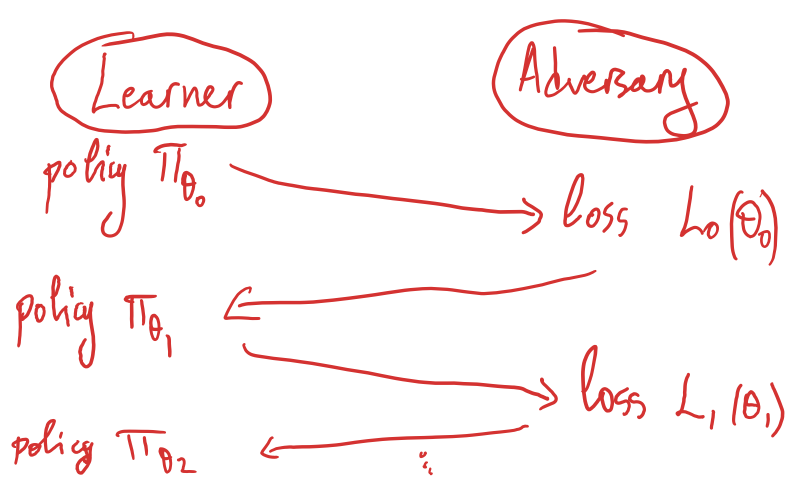
\[
r_N = \frac{1}{N} \sum_{i=1}^{N} L_i(\theta_i) - \min_{\theta \in \Theta} \left[ \frac{1}{N} \sum_{i=1}^{N} L_i(\theta) \right]
\]
\(\qquad \qquad \quad \big\uparrow\)
\(\qquad \quad \big\uparrow\)
No-regret: \(\lim_{N \to \infty} r_N = 0\)
Another way to say this: a no-regret online algorithm is one that outputs a sequence of policies \(\pi_1, \ldots, \pi_N\) such that the average loss with respect to the best-in-hindsight policy goes to 0 as \(N \to \infty\)
DAgger is a no-regret online learning algorithm
No-Regret Online Learners
Intuition: No matter what the distribution of input data, your online policy/classifier will do asymptotically as well as the best-in-hindsight policy/classifier.
\[
r_N = \frac{1}{N} \sum_{i=1}^{N} L_i(\theta_i) - \min_{\theta \in \Theta} \left[ \frac{1}{N} \sum_{i=1}^{N} L_i(\theta) \right]
\]
\(\qquad \qquad \quad \big\uparrow\)
\(\qquad \quad \big\uparrow\)
No-regret: \(\lim_{N \to \infty} r_N = 0\)
We can see Dagger as an adversarial game between the imitation learner (policy) and an adversary (environment):
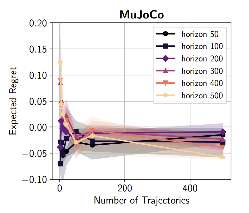
Is the quadratic regret in horizon unavoidable for behavioral cloning? No
Is the quadratic regret in horizon unavoidable for behavioral cloning? No
• Dagger’s analysis uses 0-1 loss to show quadratic regret in horizon for BC. It also only considers deterministic and linear policies.
• If instead we use log-loss BC:
\[
\hat{\pi} = \arg\min_{\pi \in \Pi} \left[ -\sum_{i=1}^{N} \sum_{t=1}^{T} \log \pi(a_t^i | x_t^i) \right]
\]
and we normalize the reward then
• BC can be shown to have linear regret in horizon, even for neural network policies.
Today’s agenda
• Administrivia
• Topics covered by the course
• Behavioral cloning
• Imitation learning
• Teleoperation interfaces for manipulation
• Imitation via multi-modal generative models (diffusion policy)
• (Time permitting) Query the expert only when policy is uncertain
Appendix 2: Why do behavioral cloning errors accumulate quadratically? Efficient reductions for imitation learning. Ross & Bagnell, AISTATS 2010.
Appendix 3: Types of Uncertainty & Query-Efficient Imitation
Let’s revisit the two main ideas from query-efficient imitation:
1. DropoutDAgger:
2. SHIV, SafeDagger, MMD-IL:
Need to review a few concepts about different types of uncertainty.
Biased Coin
\[
p(\text{heads}_3 \mid \underbrace{\text{heads}_1, \text{heads}_2}_{\textbf{observations}}) = ?
\]
Biased Coin
\[
p(\text{heads}_3 \mid \text{heads}_1, \text{heads}_2) = \int p(\text{heads}_3 \mid \theta) \underbrace{p(\theta \mid \text{heads}_1, \text{heads}_2)}_{\textbf{how biased is the coin?}} d\theta
\]
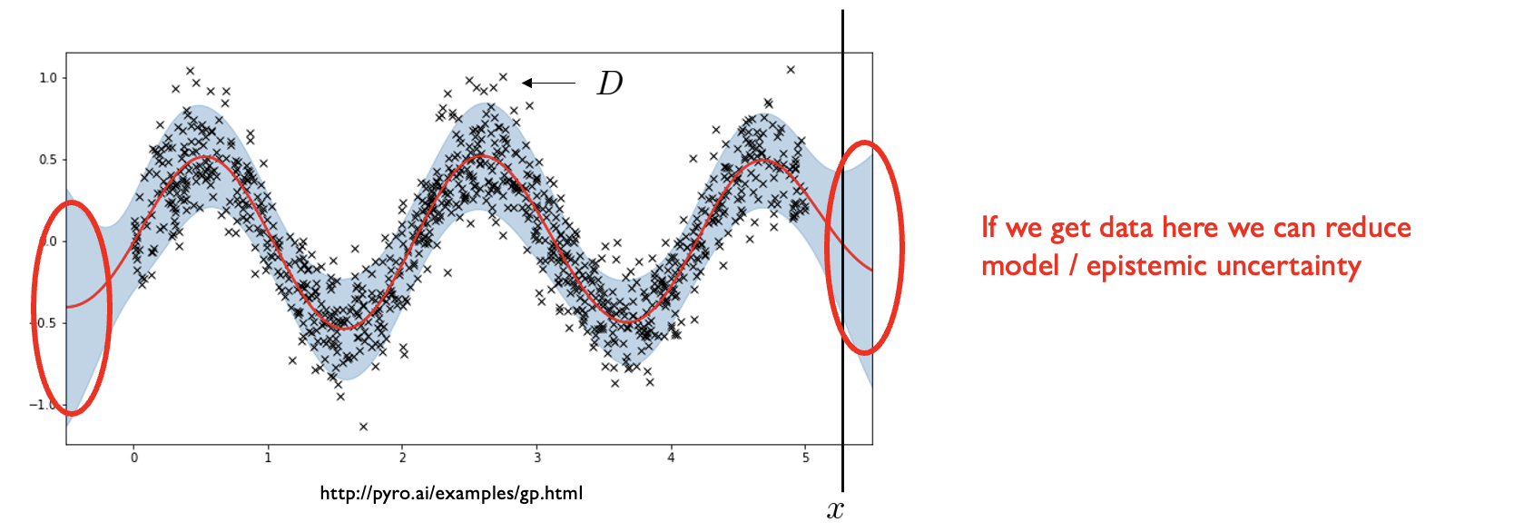
Induces uncertainty in the model, or epistemic uncertainty,
Biased Coin
\[
p(\text{heads}_3 \mid \text{heads}_1, \text{heads}_2) = \int p(\text{heads}_3 \mid \theta) p(\theta \mid \text{heads}_1, \text{heads}_2) d\theta
\]
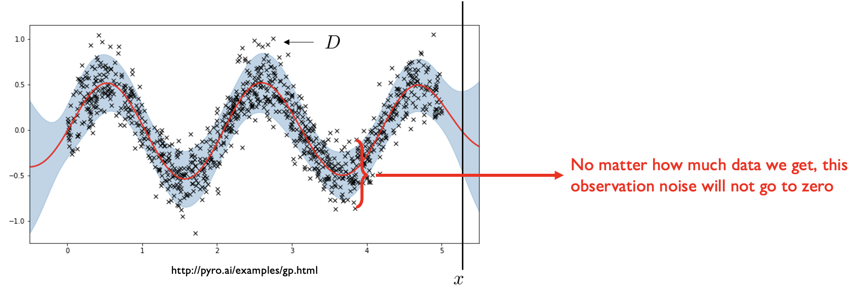
Q: Even if you eventually discover the true model, can you predict if the next flip will be heads?
A: No, there is irreducible uncertainty / observation noise in the system. This is called aleatoric uncertainty.
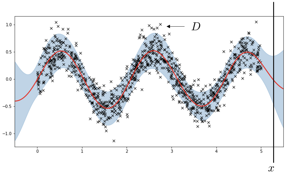
Gaussian Process Regression
\(p(\text{y} \mid \text{x}, \text{D}) = ?\)
Gaussian Process Regression
\[
p(\text{y} \mid \text{x}, \text{D}) = \int p(\text{y} \mid f) {p(f \mid x, D)} df
\]
\(f \mid x, D \sim \mathcal{N}(f; 0, K) \qquad\) Zero mean prior over functions
\(y \mid f \sim \mathcal{N}(y; f, \sigma^2) \qquad \quad\) Noisy observations
Gaussian Process Regression
\[
p(\text{y} \mid \text{x}, \text{D}) = \int p(\text{y} \mid f) {p(f \mid x, D)} df
\]
\(f \mid x, D \sim \mathcal{N}(f; 0, K) \qquad\) Zero mean prior over functions
\(y \mid f \sim \mathcal{N}(y; f, \sigma^2) \qquad \quad\) Noisy observations
Gaussian Process Regression
\[
p(\text{y} \mid \text{x}, \text{D}) = \int p(\text{y} \mid f) {p(f \mid x, D)} df
\]
\(f \mid x, D \sim \mathcal{N}(f; 0, K) \qquad\) Zero mean prior over functions
\(y \mid f \sim \mathcal{N}(y; f, \sigma^2) \qquad \quad\) Noisy observations
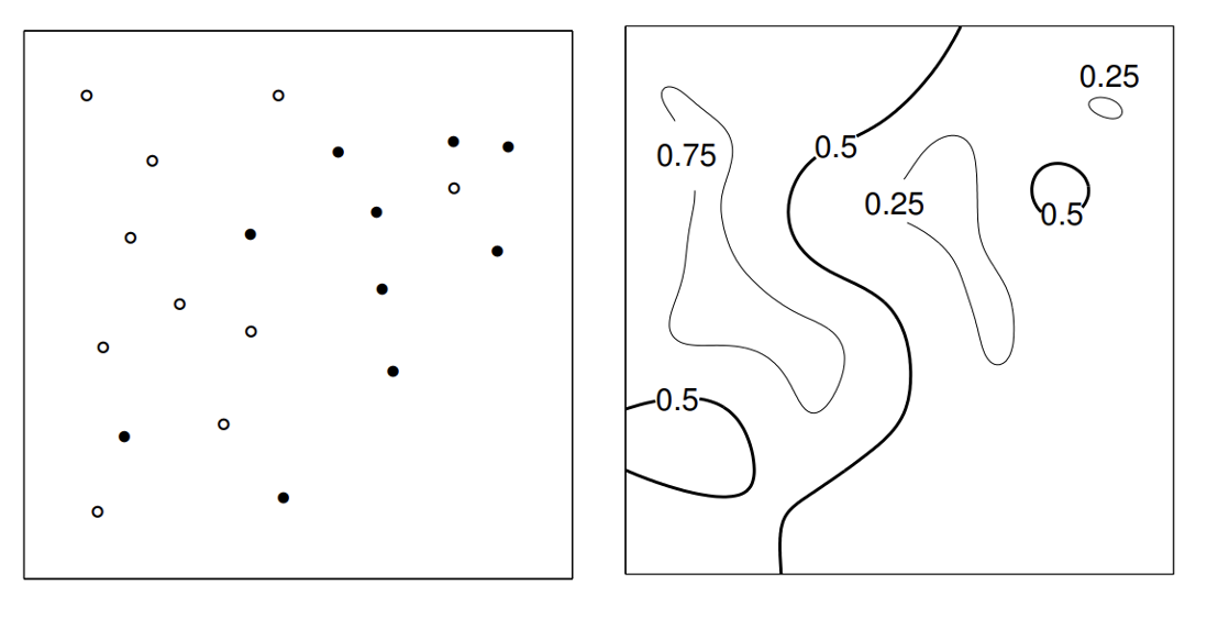
Gaussian Process Classification
GP handles uncertainty in f by averaging
Model Uncertainty in Neural Networks
Want \(p(y|x, D) = \int p(y|x, f) \, p(f|D) \, df\)
But easier to control network weights \(p(y|x, D) = \int p(y|x, w) \, \underline{\color{red} p(w|D)} \, dw\)
\(\LARGE \color{red}\nearrow\) approximates
\[
q(y|x) = \int p(y|x, w) q_{\theta^*}(w) dw
\]
\(\color{red} \LARGE \big\uparrow\) Variational inference
\[
\theta^* = \arg\min_{\theta} KL(q_{\theta}(w) || p(w|D)) \quad \color{red} \LARGE \longleftarrow
\]
How do we represent posterior over network weights?
Main ideas:
Use an ensemble of networks trained on different copies of D (bootstrap method)
Use an approximate distribution over weights (Dropout, Bayes by Backprop, …)
Use MCMC to sample weights