CSC2626 Imitation Learning for Robotics
Week 5: Imitation as Program Induction and Modular Decomposition of Demonstrations
Recurrent neural network (RNN)
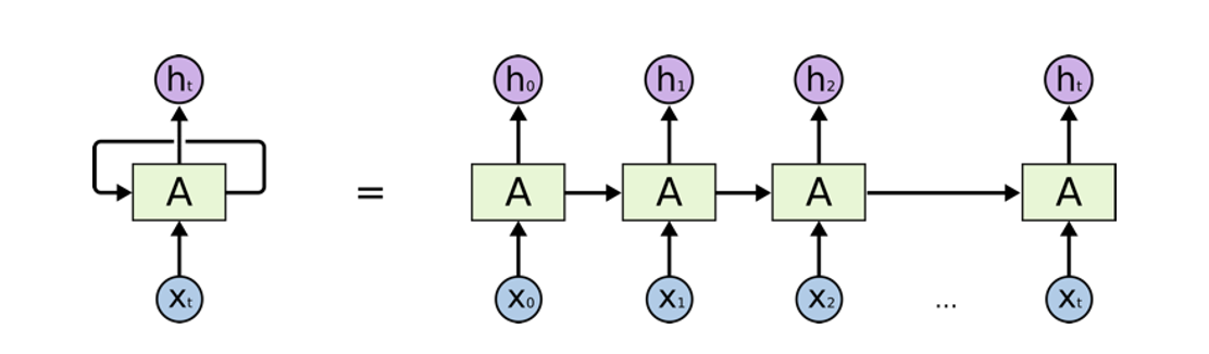
• RNN is a neural network with feedback
• Hidden state is to capture history information and current state of the network
Long Short Term Memory (LSTM)
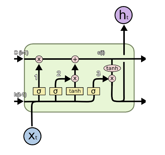
• LSTM is a special kind of RNN
• Gates are used to control information flow. Just like a valve
Model
The NPI core is a LSTM network that learns to represent and execute programs given their execution traces
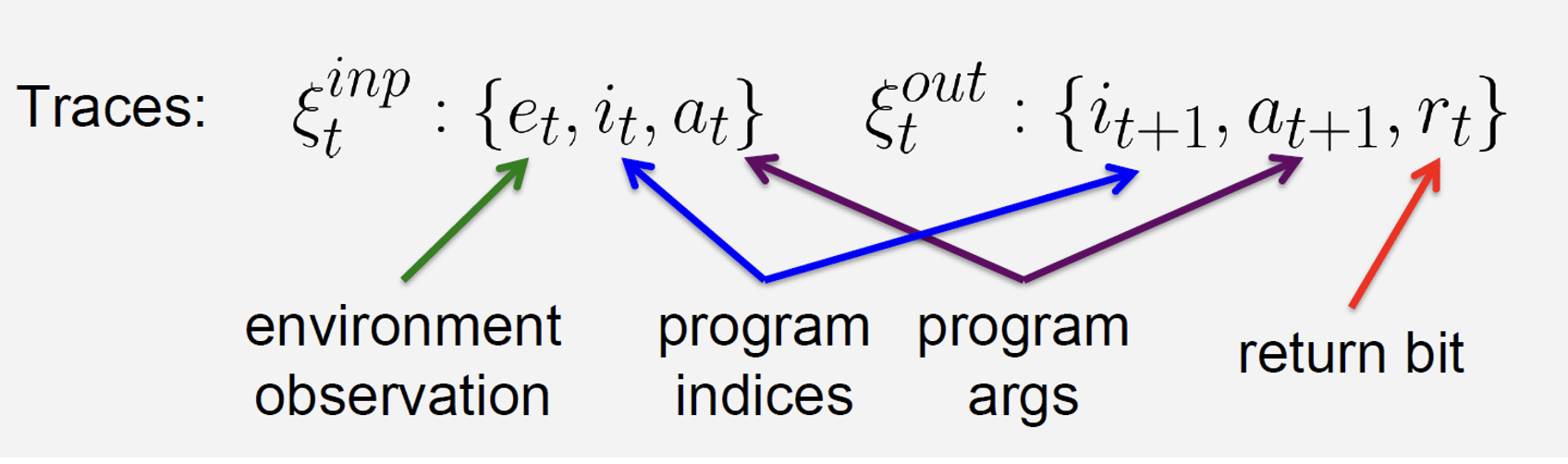
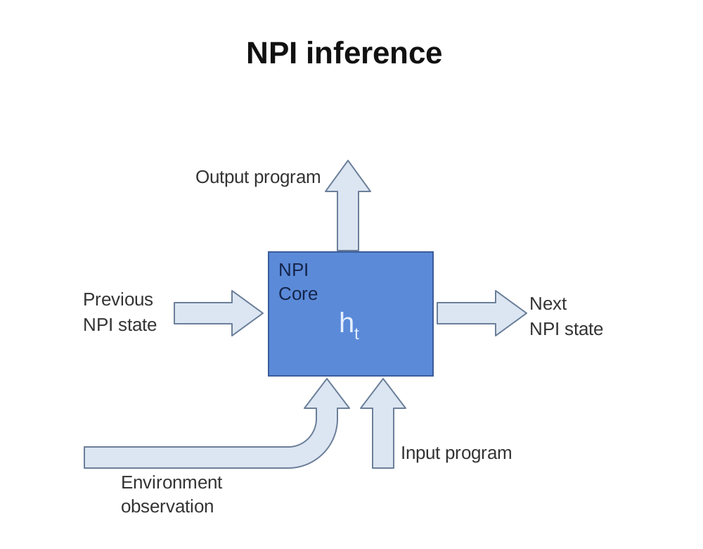
Algorithm - inference
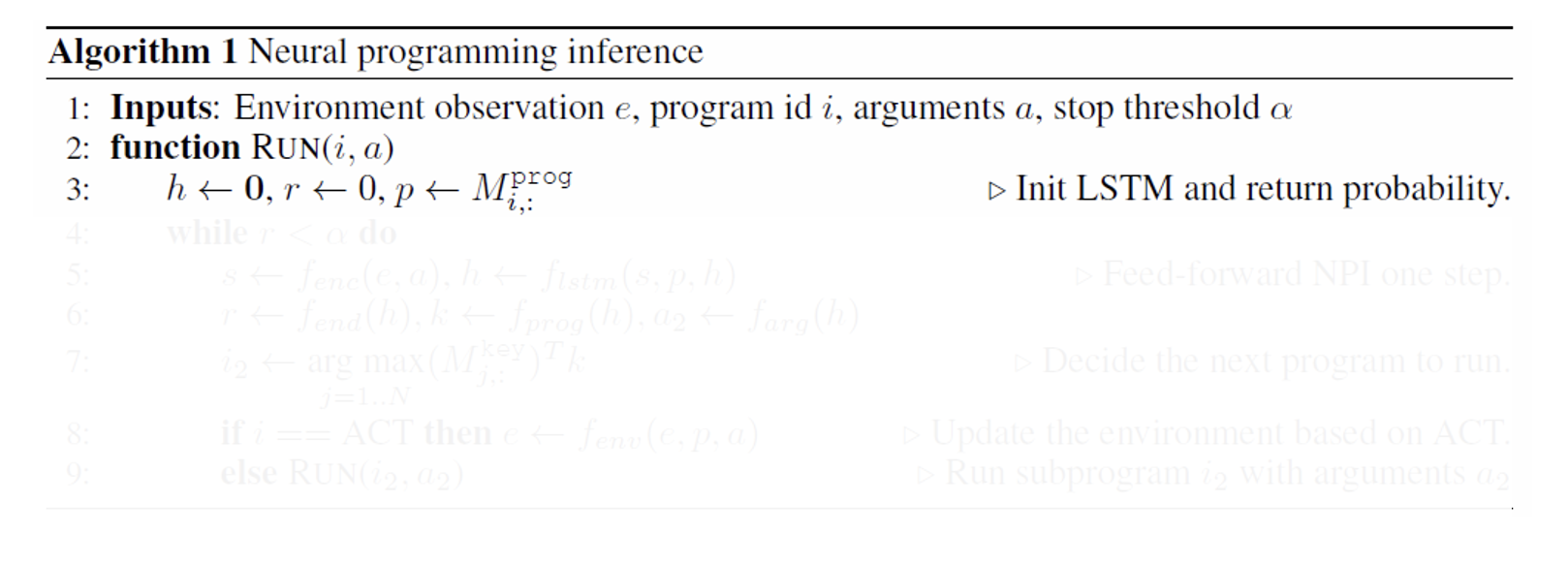
Line 3: \(𝑀^{𝑝𝑟𝑜𝑔}\) and \(𝑀^{𝑘𝑒𝑦}\) are memory banks to store program embeddings and program keys
Algorithm - inference
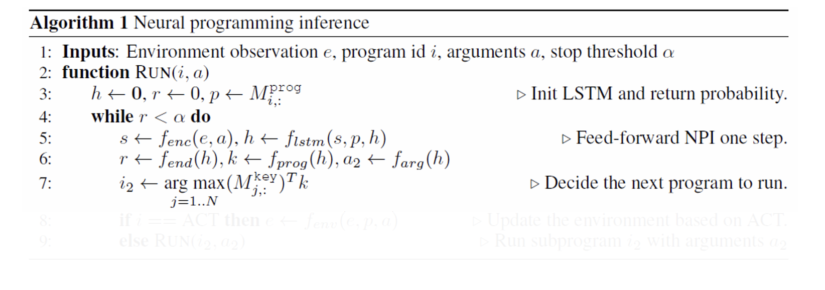
Line 7: \((𝑀_{𝑗,}^{𝑘𝑒𝑦})^{𝑇}𝑘\) is directly measurement for cosine similarity
Algorithm - inference
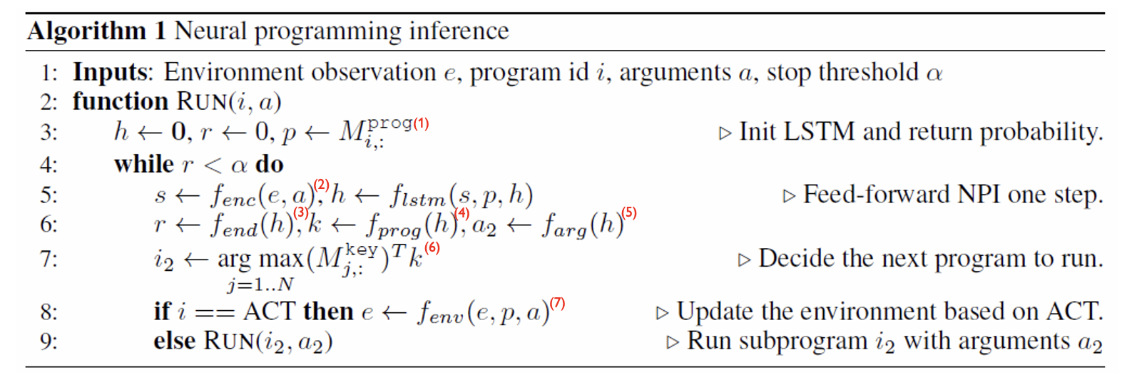
(1): \(𝑀^{𝑝𝑟𝑜𝑔}\) and \(𝑀^{𝑘𝑒𝑦}\) are memory storing program embeddings and program keys
(2): \(𝑓_{𝑒𝑛𝑐}\) is a domain-specific encoder (for different tasks, have different encoders)
(3): \(𝑓_{𝑒𝑛𝑑}\) is to calculate the probability of finishing the program
(4): \(𝑓_{𝑝𝑟𝑜𝑔}\) is to retrieve the next program key from memory
(5): \(𝑓_{𝑎𝑟𝑔}\) is to return the next program’s arguments
(6): \((𝑀_{𝑗,}^{𝑘𝑒𝑦})^{𝑇}𝑘\) is to measure cosine similarity
(7): \(𝑓_{env}\) is a domain-specific transition mapping
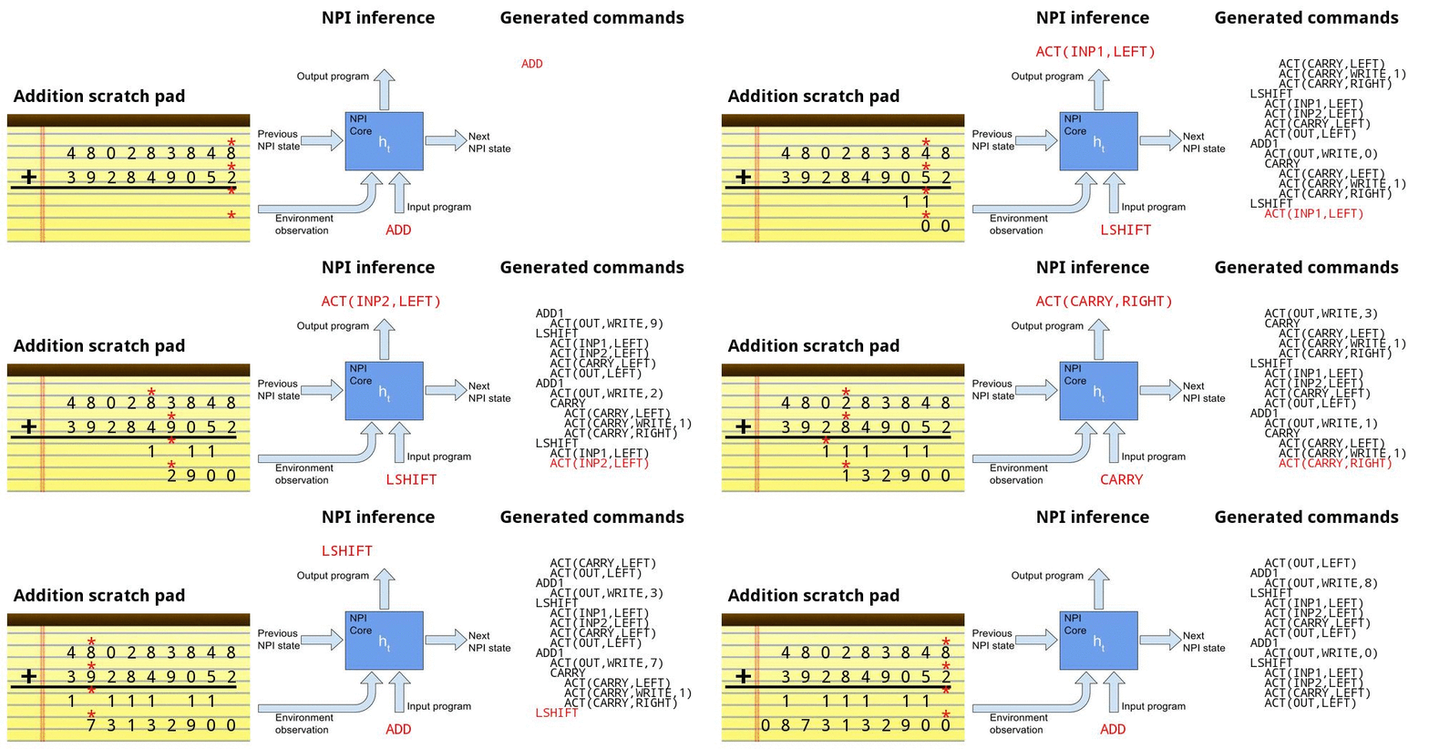
Adding numbers together
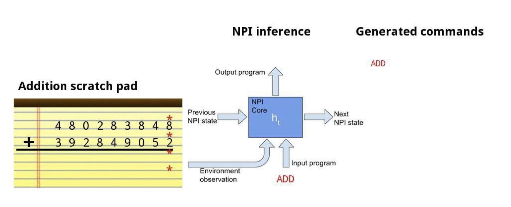
Addition demo
Bubble sort
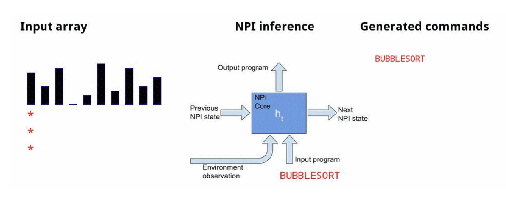
Sorting demo
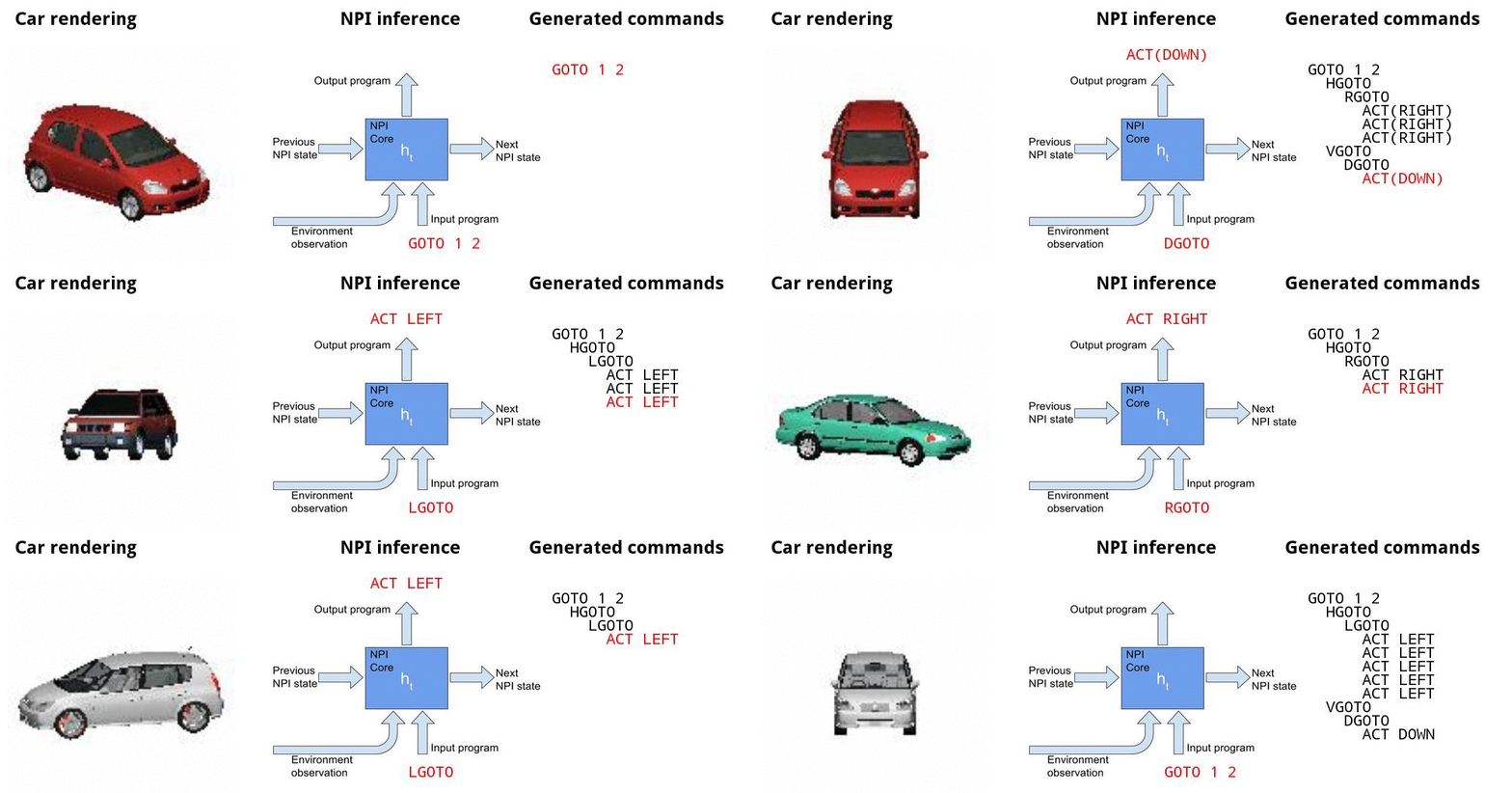
Canonicalizing 3D models
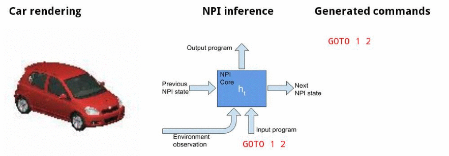
Canonicalizing demo
Data Efficiency - Sorting
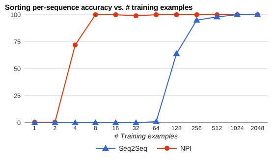
• Seq2Seq LSTM and NPI used the same number of layers and hidden units.
• Trained on length up to 20 arrays of single-digit numbers.
• NPI benefits from mining multiple subprogram examples per sorting instance, and additional parameters of the program memory.
Generalization - Sorting
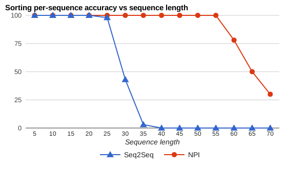
• For each length up to 20, they provided 64 example bubble sort traces, for a total of 1216 examples.
• Then, they evaluated whether the network can learn to sort arrays beyond length 20
Generalization - Adding
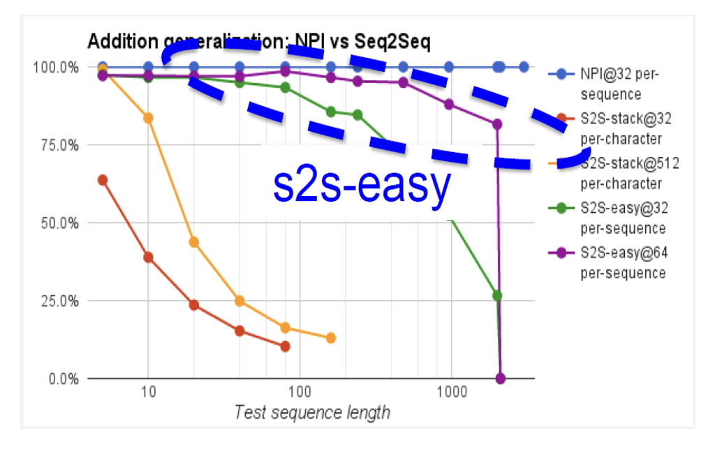
• NPI trained on 32 examples for sequence length up to 20
• s2s-easy trained on twice as many examples as NPI (purple curve)
• s2s-stack trained on 16 times more examples than NPI (orange curve)
Generalization - Adding
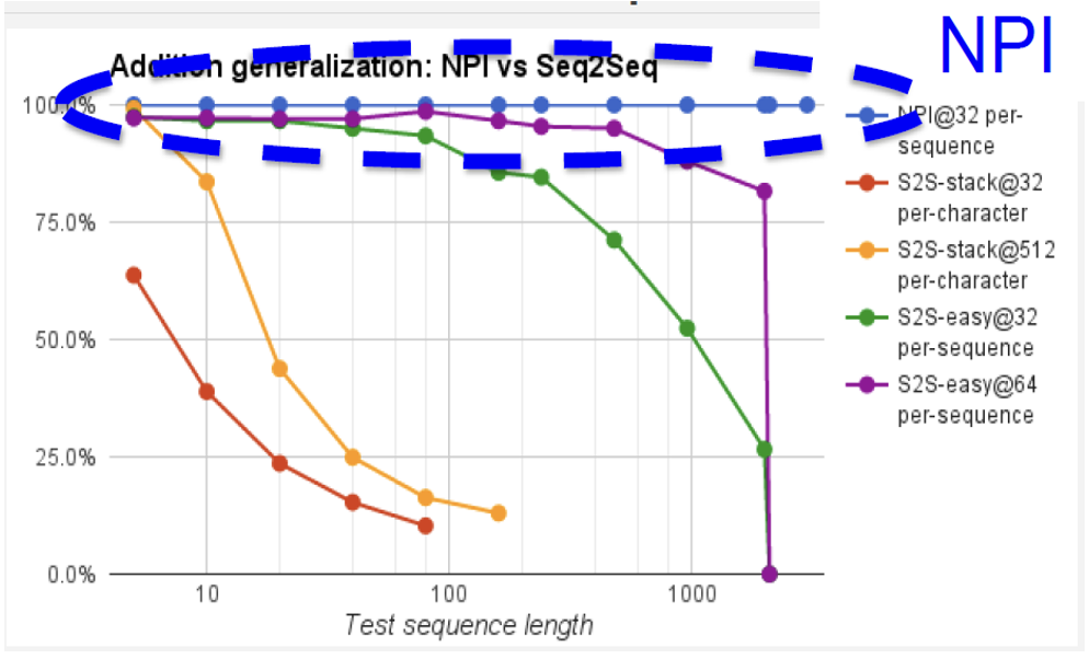
• NPI trained on 32 examples for sequence length up to 20
• s2s-easy trained on twice as many examples as NPI (purple curve)
• s2s-stack trained on 16 times more examples than NPI (orange curve)
Learning New Programs with a Fixed NPI Core
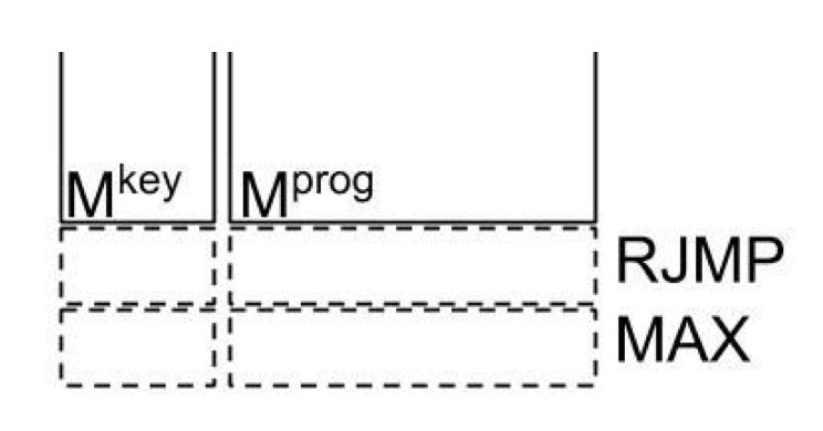
Only the memory slots of
the new program are updated!
All other weights are
fixed!
Protocol:
• Randomly initialize new program vectors in memory
• Freeze core and other program vectors
• Backpropagate gradients to new program vectors
Quantitative Results
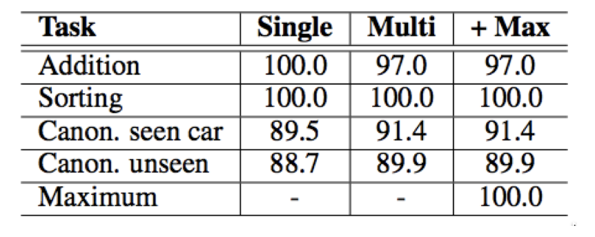
• Numbers are per-sequence % accuracy
• + Max: indicates performance after addition of MAX program to memory
• “unseen” uses a test set with disjoint car models from the training set
Followup work: AlphaNPI (training NPI without execution traces)
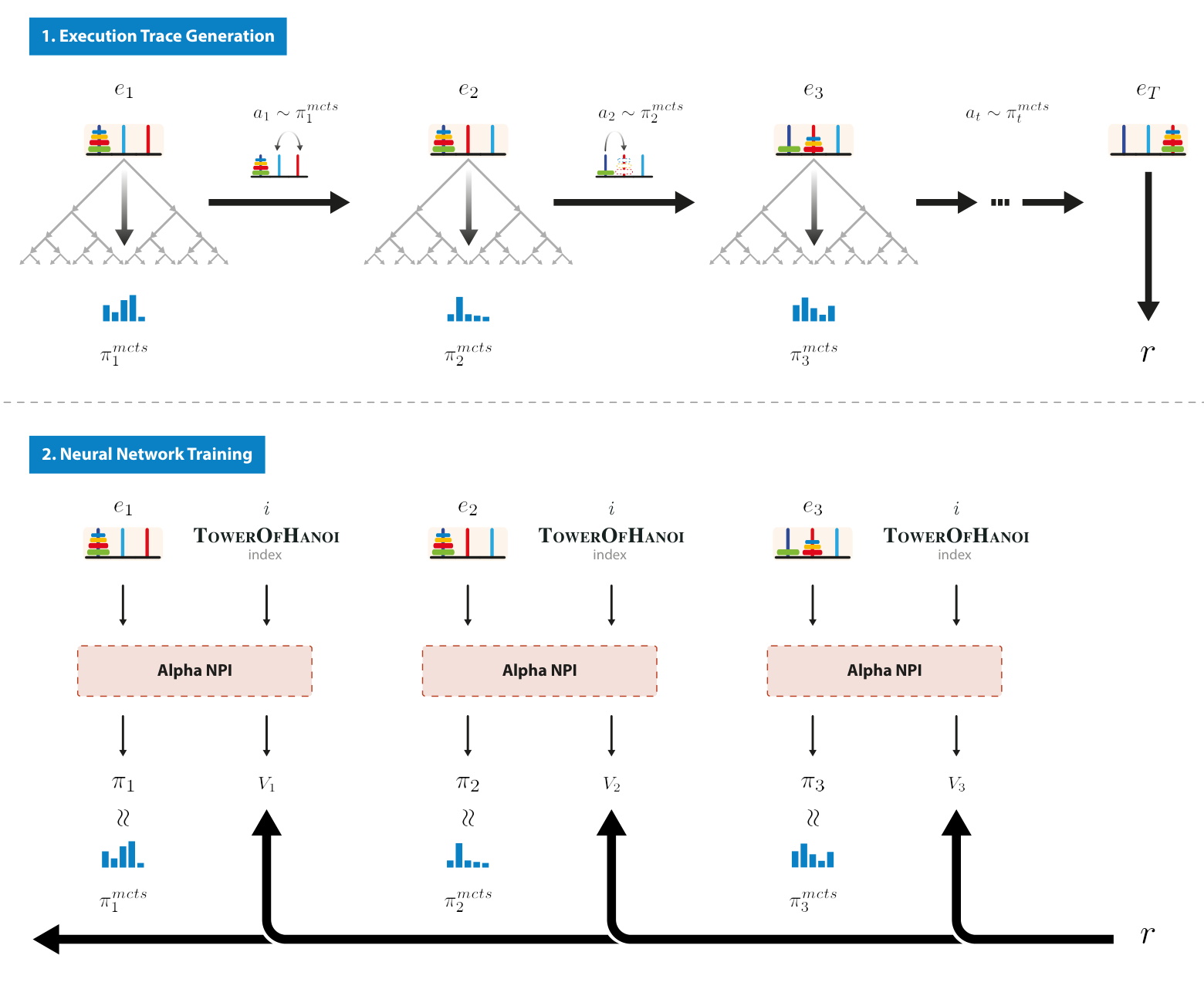
NPI needs full execution traces. AlphaNPI only needs a specification: a hierarchy of programs, each with pre- and post-conditions
Sparse reward: 1 if the post-conditions hold when the program calls STOP, 0 otherwise
NPI becomes an actor-critic (policy \(\pi\), value \(V\)), trained as in AlphaZero: MCTS gives an improved policy \(\pi^{mcts}\), and the loss is \(-\pi^{mcts\top} \log \pi + (V - r)^2\)
Recursive MCTS: calling a learned program builds a new search tree for it
Recursive bubble sort trained on lists of length ≤ 4: 100% on length 100 with MCTS, 10% with the network alone. Tower of Hanoi trained on 2 disks: 100% on 12 disks
Learning Compositional Neural Programs with Recursive Tree Search and Planning, Pierrot et al, NeurIPS 2019. https://arxiv.org/abs/1905.12941
How the algorithm works
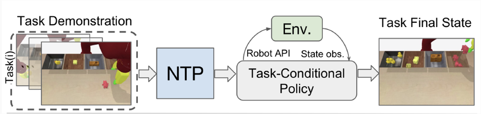
- Task Demonstration: state trajectory, first/third-person video demonstrations, or a list of language instructions.
- Task-Conditional Policy: a neural program.
- Using callable primitive actions to interact with the environment.
How the algorithm works
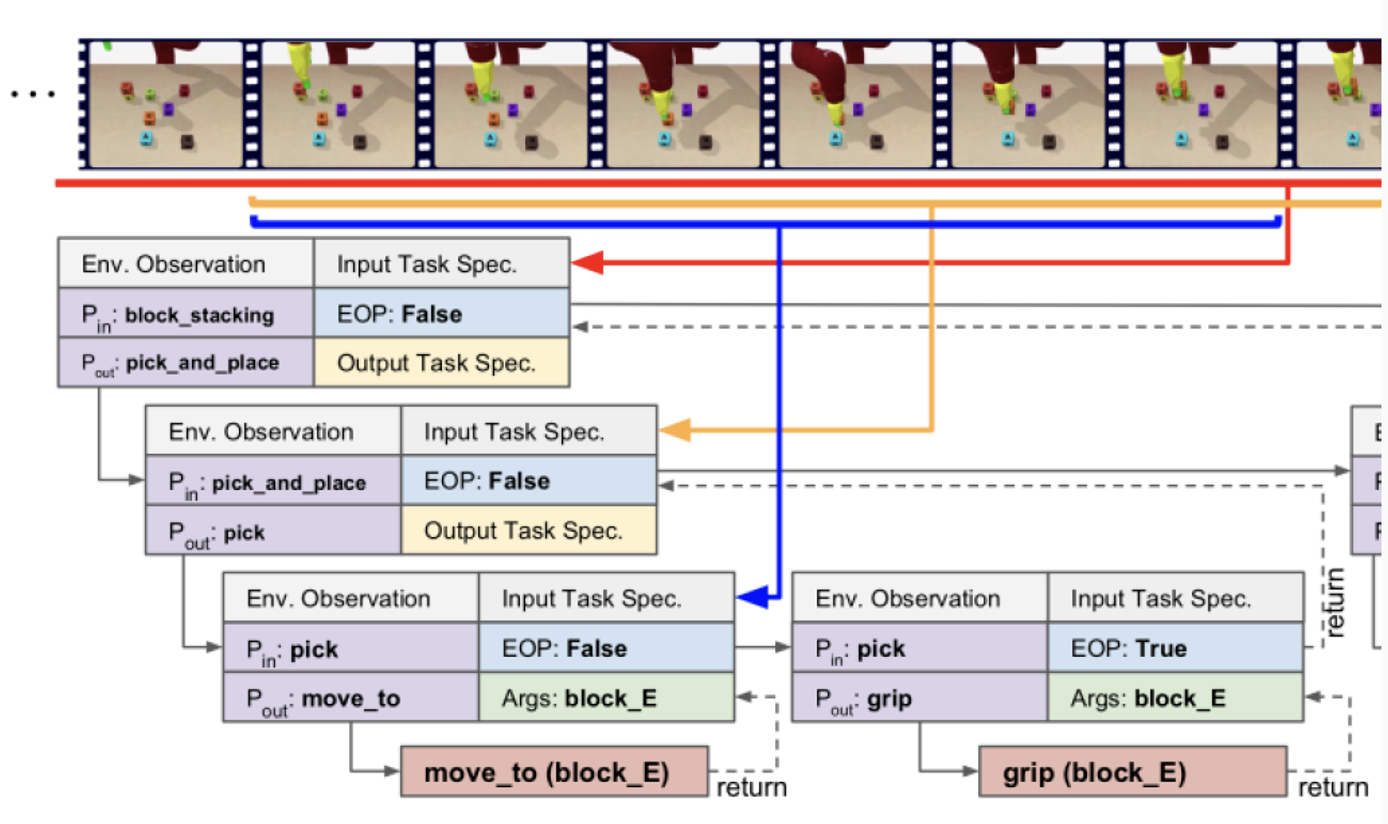
Top-level program block_stacking is recursively decomposed to bottom-level API move_to and grip.
Implementation: Neural Task Programming
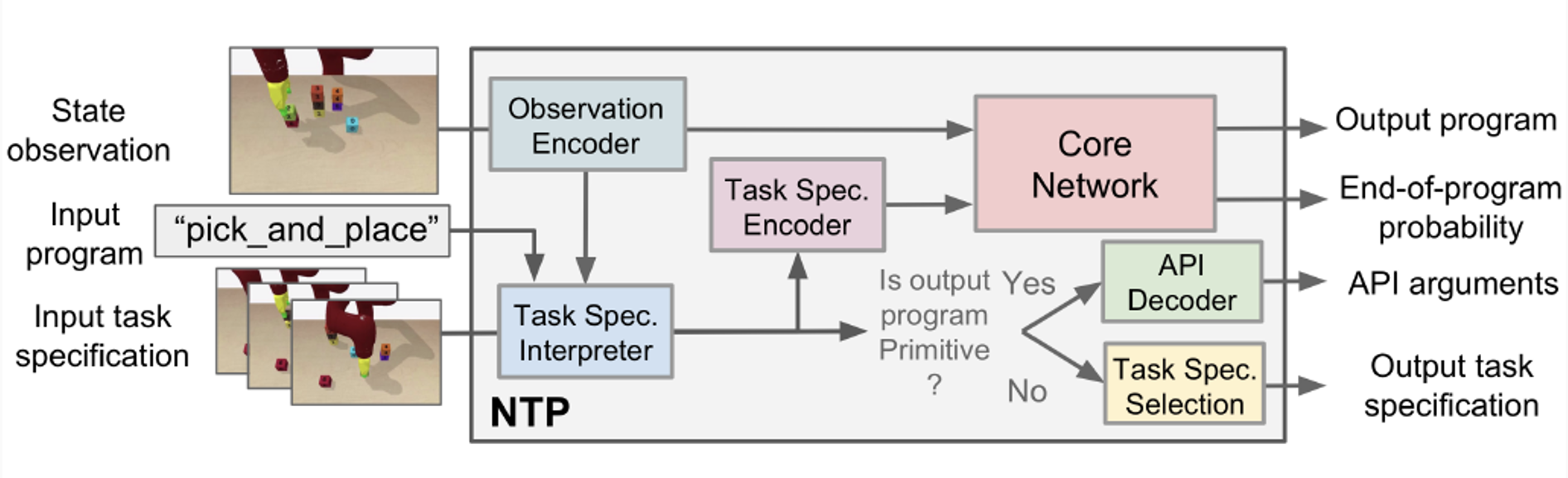
- Observation Encoder: observation \(o_i \Rightarrow\) state representation \(s_i\)
- Task Spec. Interpreter: \(\Rightarrow\) API arguments \(a_i\) or task spec. \(\psi_{i+1}\)
- Task Spec. Encoder: task spec. \(\psi_i \Rightarrow\) vector space \(\phi_i\)
- Core Network: \(s_i, P_i, \phi_i \Rightarrow P_{i+1}, r_i\)
Experiments: Setup
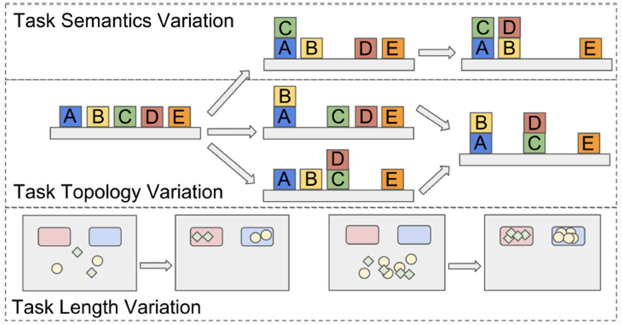
- Generalization in 3 variations: semantics, topology, and length.
- Using image-based input without access to ground truth state.
- Working in real-world tasks combine these variations.
→ Three tasks: Object Sorting, Block Stacking, and Table Clean-up
Experiments: Object Sorting
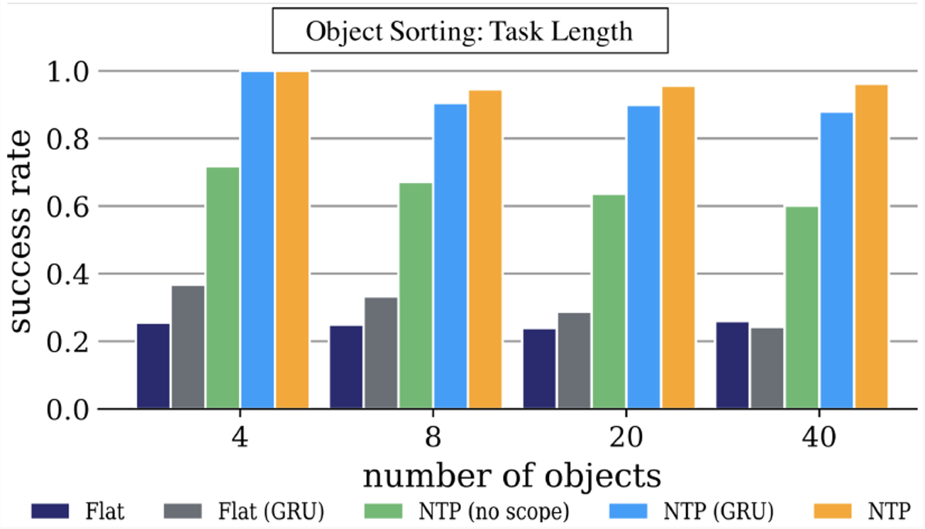
Flat: non-hierarchical model, directly predicts the primitive APls instead of calling hierarchical programs.
GRU: Gated Recurrent Unit.
Experiments: Block Stacking
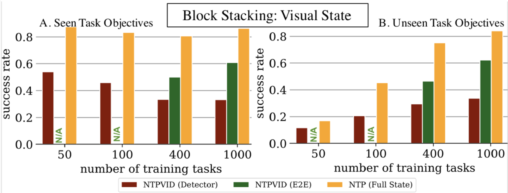
- NTPVID(E2E): Trained with only visual information.
- NTP(Full State): Trained with ground-truth hierarchical decomposition.
Experiments: Table Clean-up
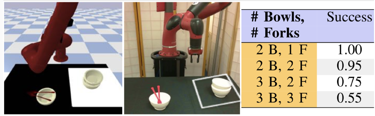
Sort plastic bowls and forks into a stack, so they can be steadily carried away.
Task variations:
- Task length: number of bowls and forks varies.
- Task topology: the ordering in which bowls are stacked varies.
Motivation – Block Stacking Task
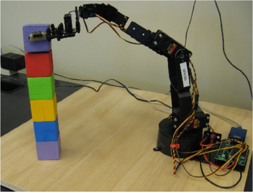
Complex tasks can often be broken down into simpler sub-tasks
Most Learning from Demonstration (LfD) algorithms can only learn a single policy for the whole task
Resulting in more complex policies, and also less reusable
Example: Block stacking task
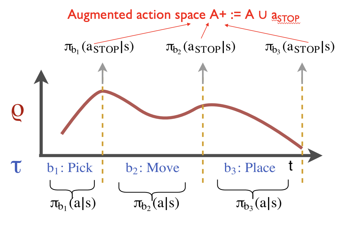
TACO: Temporal Alignment for Control
Input trajectory \(\rho=((s_1,a_1),...,(s_T,a_T))\)
Task sketch \(\tau = (b_1, b_2, . . . , b_L)\) indicating which sub-tasks are active in \(\rho\). Assume \(L \ll T\)
A path \(\zeta = (\zeta_1, \zeta_2, ..., \zeta_T )\) is a sequence of sub-tasks of the same length as the input sequence \(\rho\), describing the active sub-task \(\zeta_t\) at every time-step
\(Z_{T,\tau}\) is the set of all possible paths \(\zeta\) of length T, given a task sketch \(\tau\)
Eg. T = 6, \(\tau = (b_1, b_2, b_3), \zeta = (b_1, b_1, b_2, b_3, b_3, b_3)\)
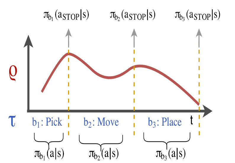
TACO: Temporal Alignment for Control
\(\alpha_1(l) = \begin{cases} \pi_{\theta_{b_1}}(a_1|s_1), & \text{if } l = 1, \\ 0, & \text{otherwise}. \end{cases}\)
\(\alpha_t(l) = \pi_{\theta_{b_l}}(a_t|s_t) \left[ \alpha_{t-1}(l-1) \pi_{\theta_{b_{l-1}}}(a_{STOP}|s_t) \right.\)
\(\left. + \alpha_{t-1}(l)(1 - \pi_{\theta_{b_l}}(a_{STOP}|s_t)) \right].\)
\(\alpha_T(L) = p(\tau, \mathbf{a}_\rho|\mathbf{s}_\rho).\)
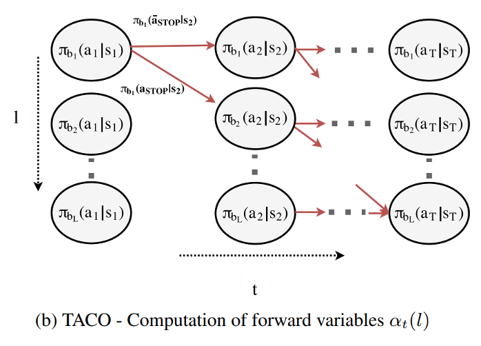
Training: Maximize \(\sum_{\rho} \log \alpha_T(L)\) over all demonstrations, w.r.t. the sub-policy parameters \(\theta=(\theta_1, ..., \theta_K)\), which define both the action policies \(\pi_{\theta_k}(a|s)\) and the stop policies \(\pi_{\theta_k}(a_{STOP}|s)\)
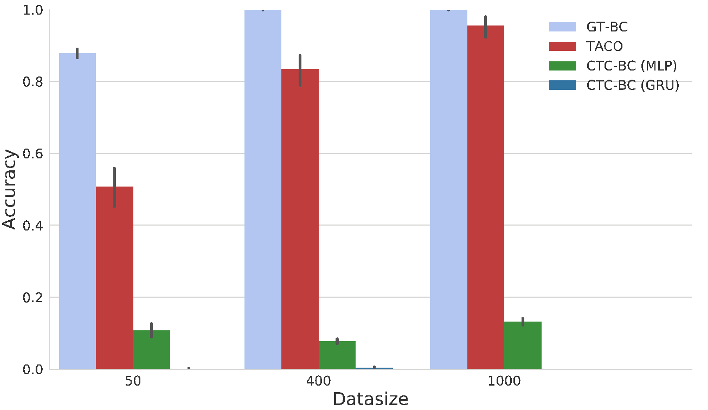
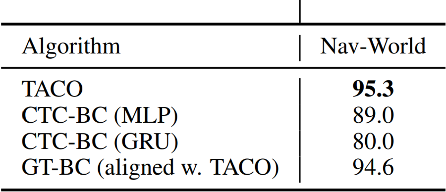
Experiments: Nav-World
Setup:
- The agent (blue) receives a route as a task sketch.
- 𝛕 = (black, green, yellow, red)
- State space: (x, y) distance from each of the destination points
- Action space: \((v_x, v_y)\) - the velocity
Training:
- Provided with state-action trajectories ⍴ and the task sketch.
- At the end of learning, the agent learns four sub-policies
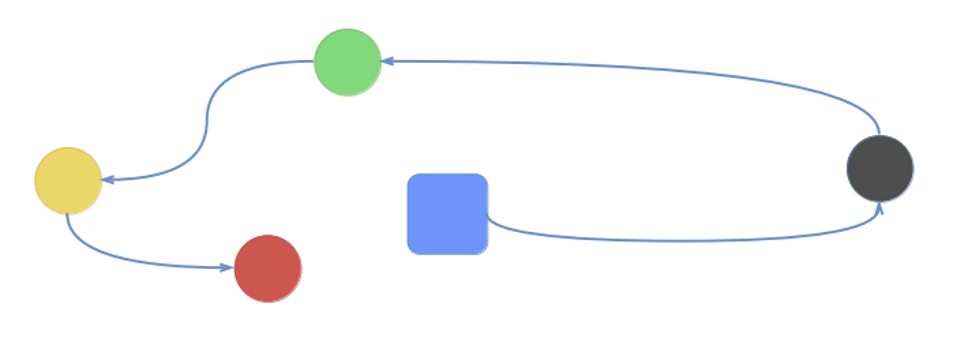
Test:
- Given an unseen task sketch.
- Considered successful if the agent visits all destinations in the correct order
Experiments: Nav-World
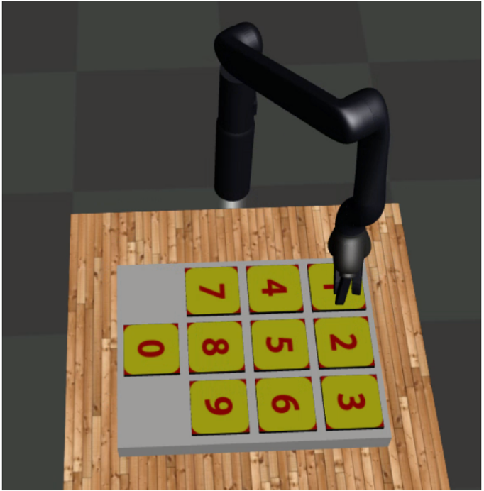
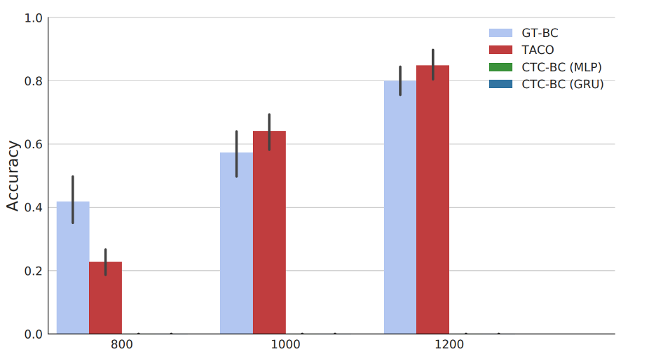
Experiments: Dial Domain
Task and Motion Planning
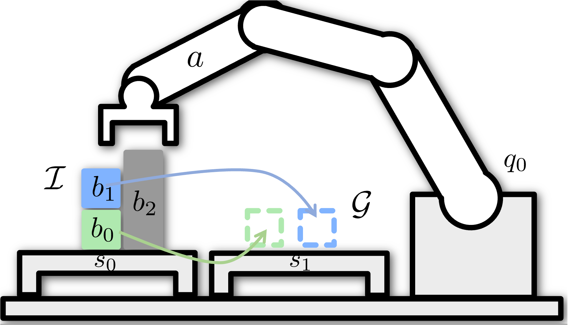
Goal: move green box and blue box on the goal surface
Problem: grey box is obstructing
Task plan:
- move grey box where it doesn’t obstruct
- move blue box on goal surface
- move green box on goal surface
Task and Motion Planning
Discrete action space: 3 objects x 4 operations
Continuous action space: 5 joint angles on the robot arm x T timesteps
find-grasp(b, hand)
place(b, hand, sur face)
find-traj(hand, goal)
collides(arm, b, objects)
\(b \in \{b_0, b_1, b_2 \}\)
Task and Motion Planning
Discrete action space: M objects x N operations
Continuous action space: 5 joint angles on the robot arm x T timesteps
find-grasp(b, hand)
place(b, hand, sur face)
find-traj(hand, goal)
collides(arm, b, objects)
pour(b, b’)
stir(b)
shake(b)
.
.
.
Task and Motion Planning
Discrete action space: M objects x N operations
Continuous action space: 5 joint angles on the robot arm x T timesteps
Discrete + Continuous Optimization
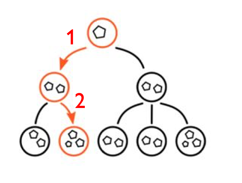
Expanding 1 and 2 requires solving continuous optimization problems with constraints
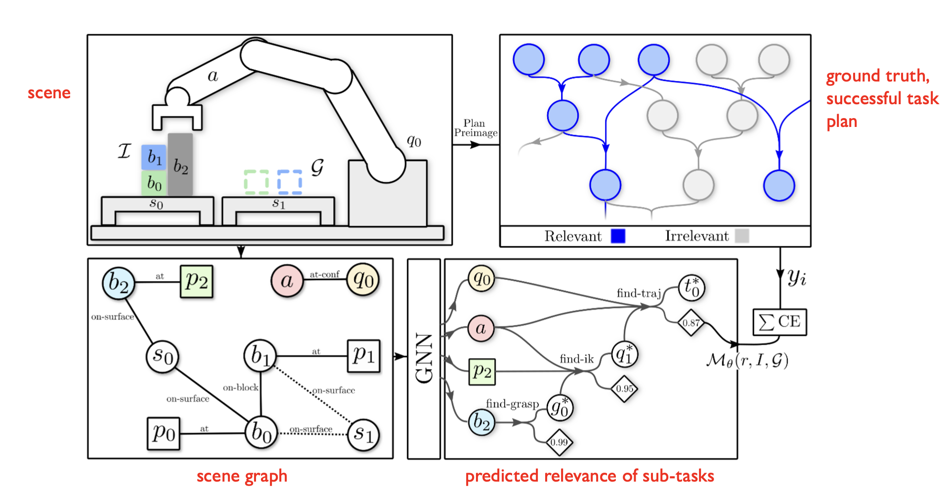
Learning to Rank Objects and Operations from Past Experience
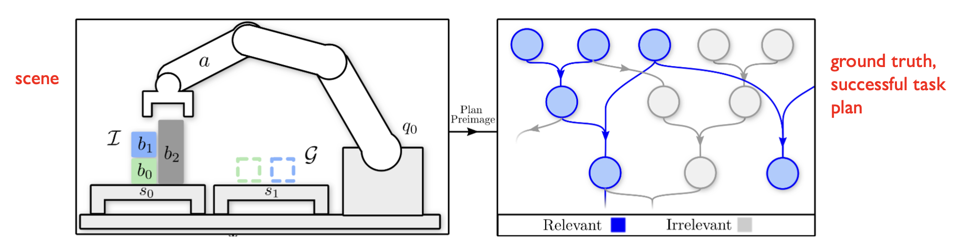
Learning to Rank Objects and Operations from Past Experience
Learned (Informed) Planner Finds Solutions Faster
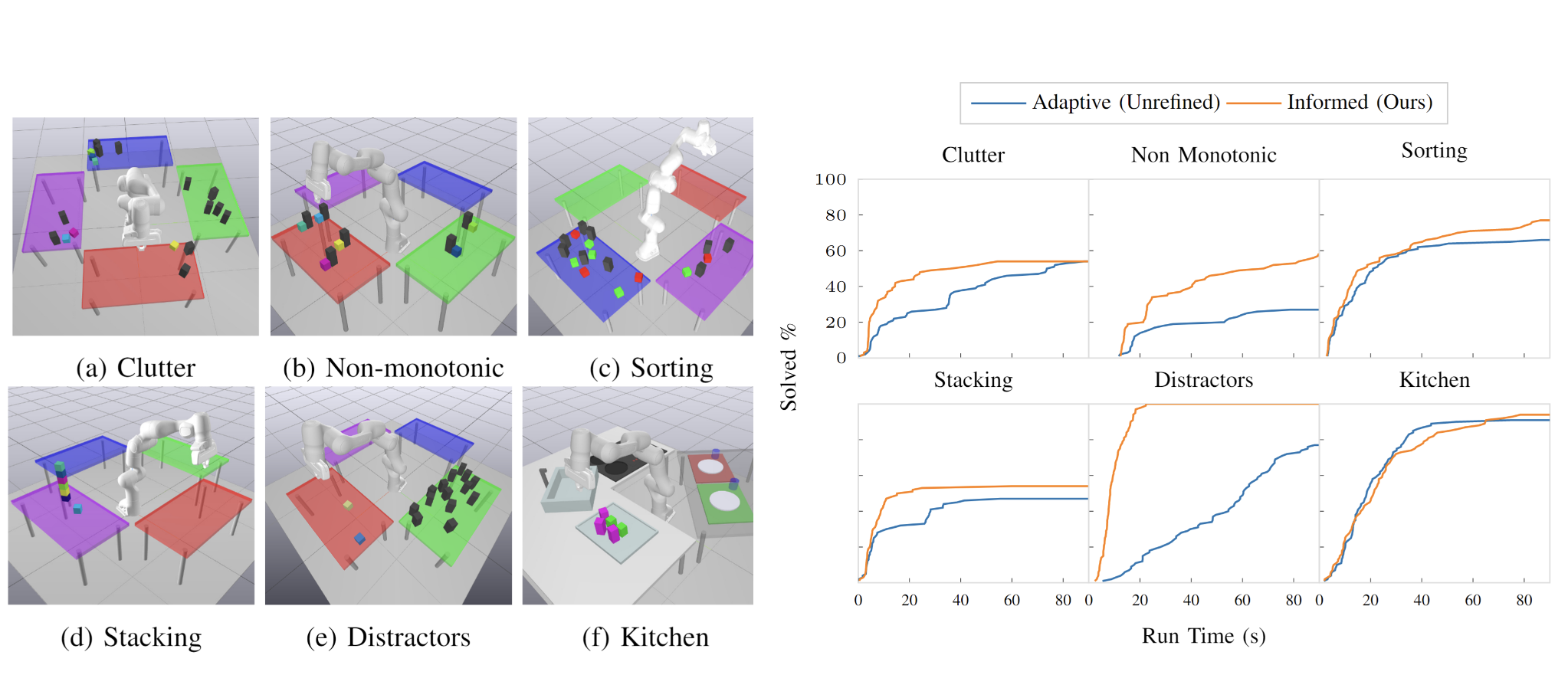
*Learning to Search in Task and Motion Planning with Streams, Khodeir et al, Robotics and Automation Letters. 2022
Motivation: who writes the planning domain?
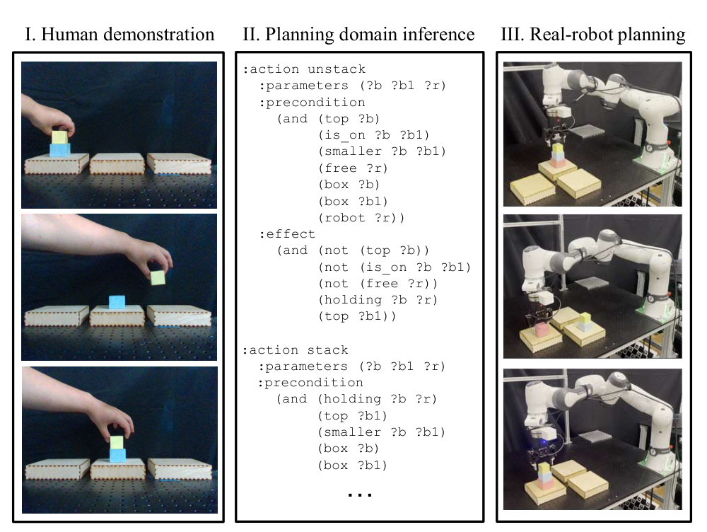
- Goal: infer the planning domain of a new task from one (or a few) human demonstrations, then plan with a standard TAMP planner
- Unlike behavioural cloning of the planner, only the domain is learned. The search is still done by the planner, which helps generalize to more objects
Predicate and action estimators
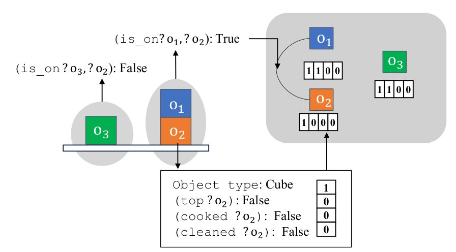
Initial and goal states as scene graphs: objects are nodes, predicates are node features and edges
Graph attention network → relevance score \(u_p, u_a \in [0, 1]\) for every predicate and action
Score of a candidate domain with predicates and actions \(\omega_\mathbf{D}\):
\[ u_\mathbf{D} = \prod_{p \in \omega_\mathbf{D}} u_p \prod_{p \notin \omega_\mathbf{D}} (1 - u_p) \prod_{a \in \omega_\mathbf{D}} u_a \prod_{a \notin \omega_\mathbf{D}} (1 - u_a) \]
The best-scoring \(\omega_\mathbf{D}^{top}\) is the initial guess. The rest are ranked by score in a priority list \(L\)
Generate-and-test domain search
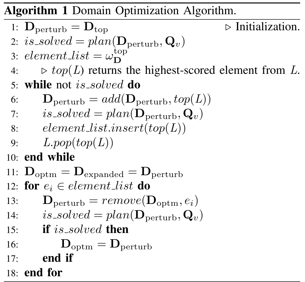
\(\omega_\mathbf{D}^{top}\) → PDDL domain \(\mathbf{D}_{top}\), using the demonstration:
- Precondition of an action: intersection of its pre-images (logical state just before the action) over all its instances
- Effect: intersection of its post-images, keeping only the predicates that changed
Expansion: add the highest-scored element of \(L\) until the domain solves all of \(\mathbf{Q}_v\)
Contraction: try removing each element. Keep the removal if \(\mathbf{Q}_v\) is still solved
Assumes that a subdomain of an incomplete domain is incomplete, and that the optimal domain is contained in any complete domain
Each
plancall queries the motion planners, which dominates the cost. A good initial guess means few calls
Results: more objects and new tasks
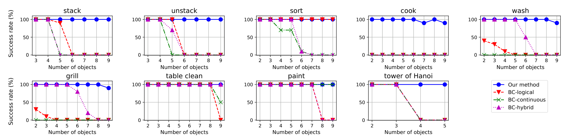
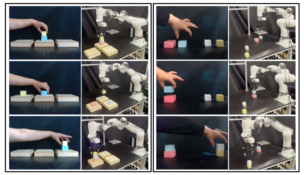
- One demonstration per task at test time. Test problems have up to 9 objects, training problems at most 4
- Behavioural cloning baselines: graph attention policies that predict the next logical action from logical, continuous or hybrid object states
- Inferred domains stay above 90% success up to 9 objects, while the baselines degrade on complex tasks
Unseen composed tasks, one demonstration each (success rate % vs. number of objects):
| Task | 3 | 4 | 5 | 6 | 7 | 8 | 9 |
|---|---|---|---|---|---|---|---|
| Cook and plate | 100 | 100 | 100 | 100 | 100 | 40 | 50 |
| Unpack and cook | 100 | 100 | 100 | 100 | 100 | 80 | 50 |
| Label | 100 | 100 | 100 | 100 | 100 | 100 | 100 |
Results: search cost and real robot experiments

What do you need for compositional generalization in diffusion planning?
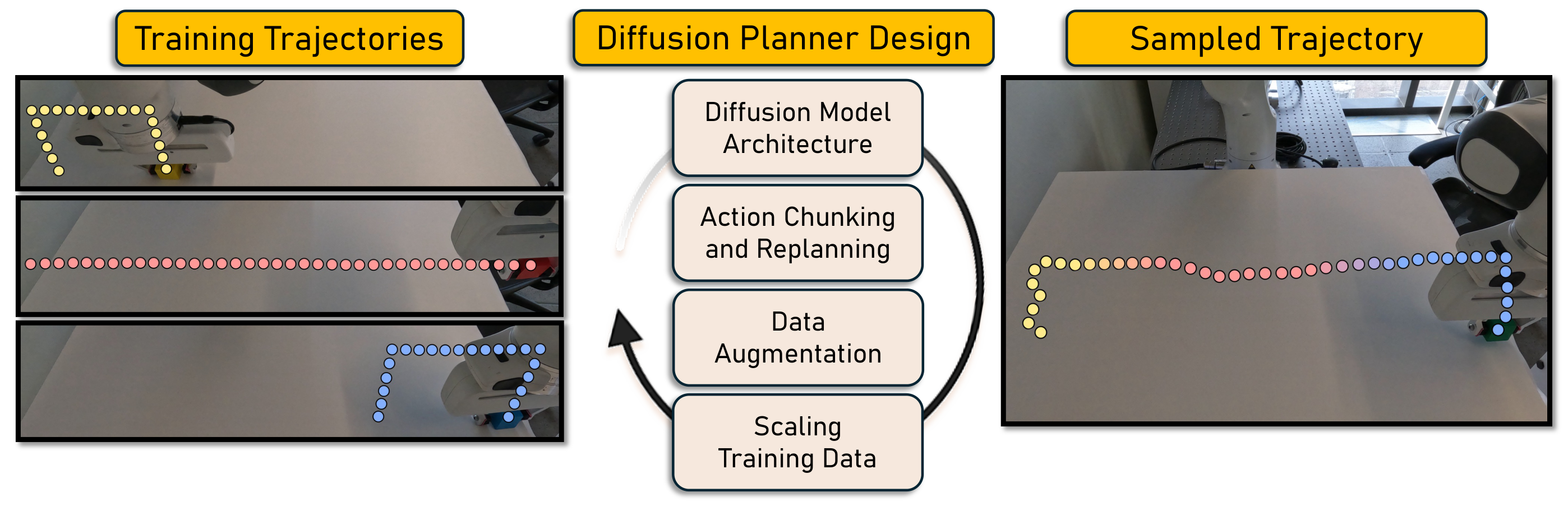
- Diffusion planners trained via imitation (generative behavioural cloning), not RL
- Compositional generalization: generating new trajectories by stitching together sub-trajectories from different demonstrations
- Which design choices enable it?
What Do You Need for Compositional Generalization in Diffusion Planning? Quentin Clark and Florian Shkurti. CoRL 2026. https://arxiv.org/abs/2505.18083
Popular diffusion planners memorize
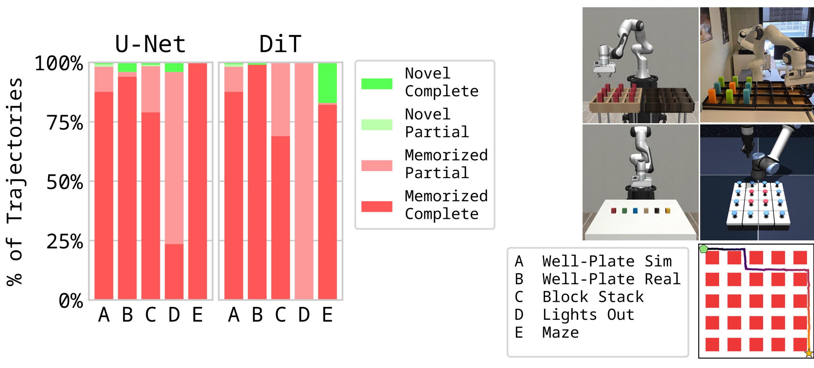
- Memorized: every sub-task of the generated trajectory appears together in a single training trajectory. Novel: requires combining parts of two or more training trajectories
- Complete: as many sub-tasks as a training trajectory. Partial: fewer
Eq-Net design
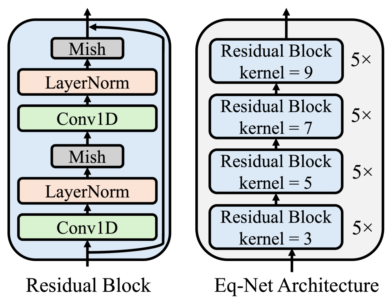
A ResNet CNN with:
- Small convolution kernels
- No max-pooling
- No indexed upsampling
✅ Local receptive fields
✅ Shift-equivariance
Eq-Net memorizes less
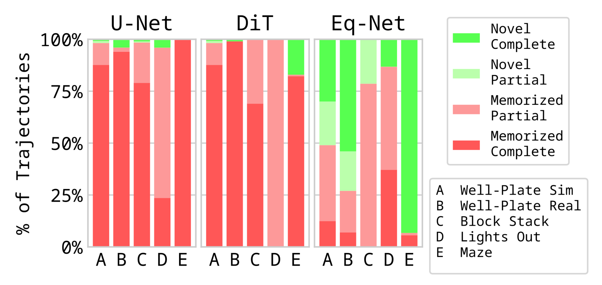
Eq-Net generates many more novel trajectories than U-Net and DiT backbones
Locality vs dataset size
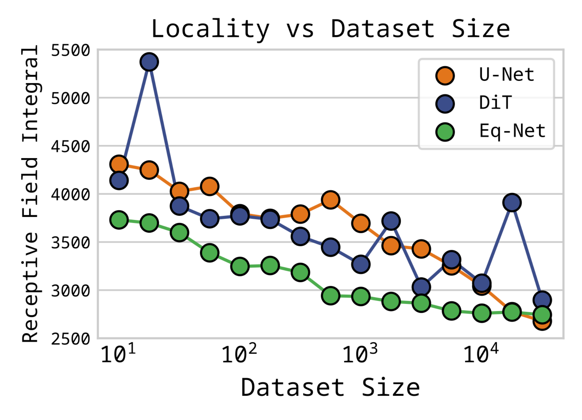
Lower receptive field integral = more local. Models trained on more data are more local, and Eq-Net is local even with little data
More data induces local receptive fields
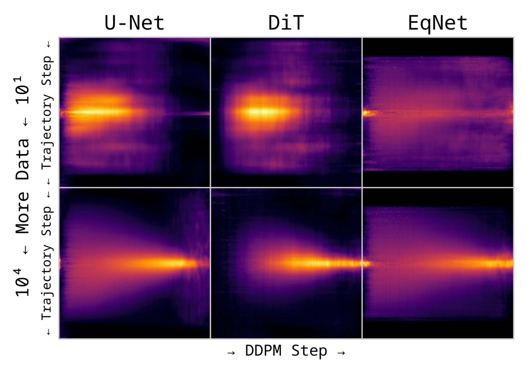
Gradient of the center state w.r.t. the trajectory
Low-data regime: large receptive fields
High-data regime: small receptive fields
Compositionality vs dataset size
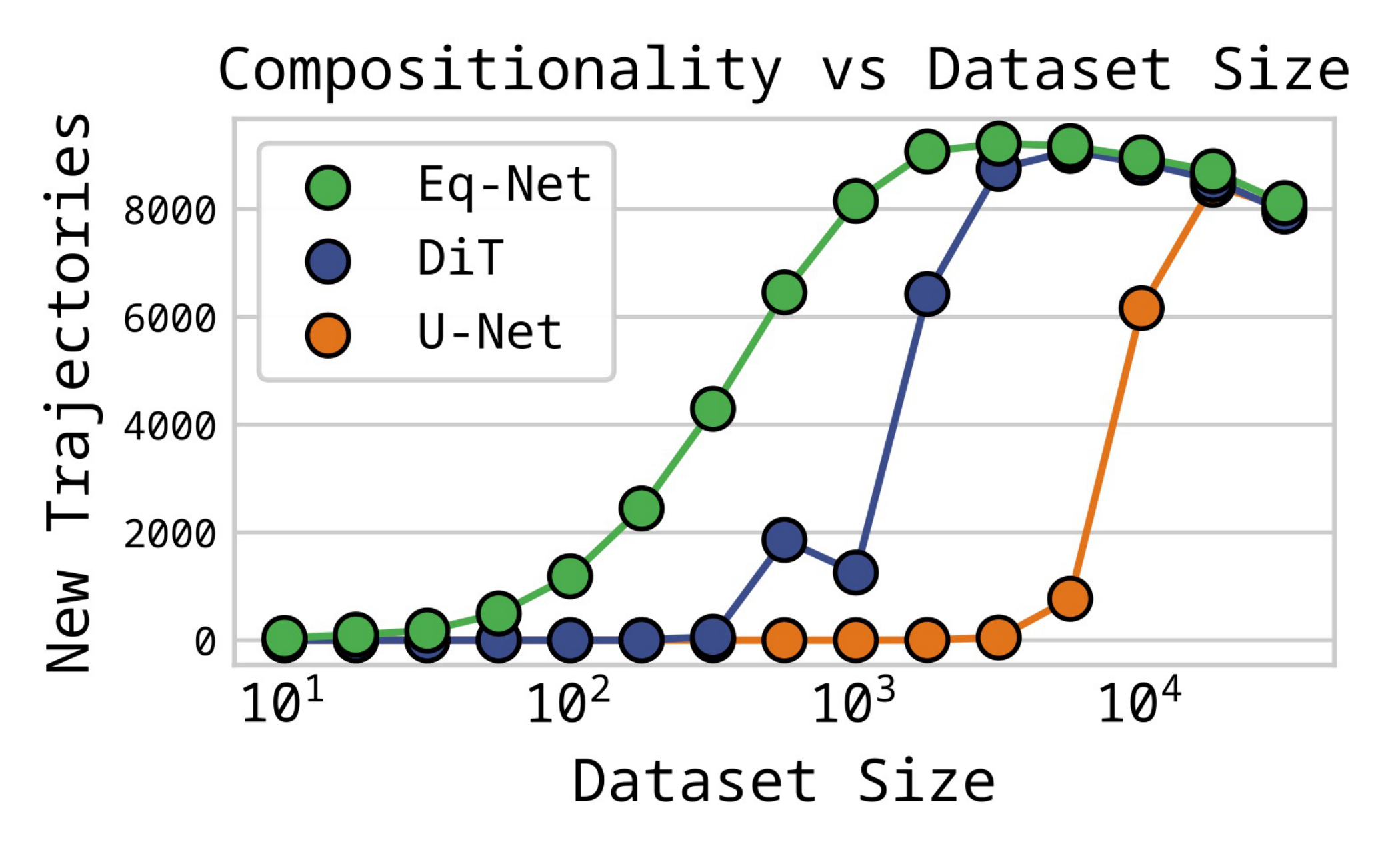
Eq-Net composes with much less data. U-Net and DiT only start composing once the dataset is large enough to make them local
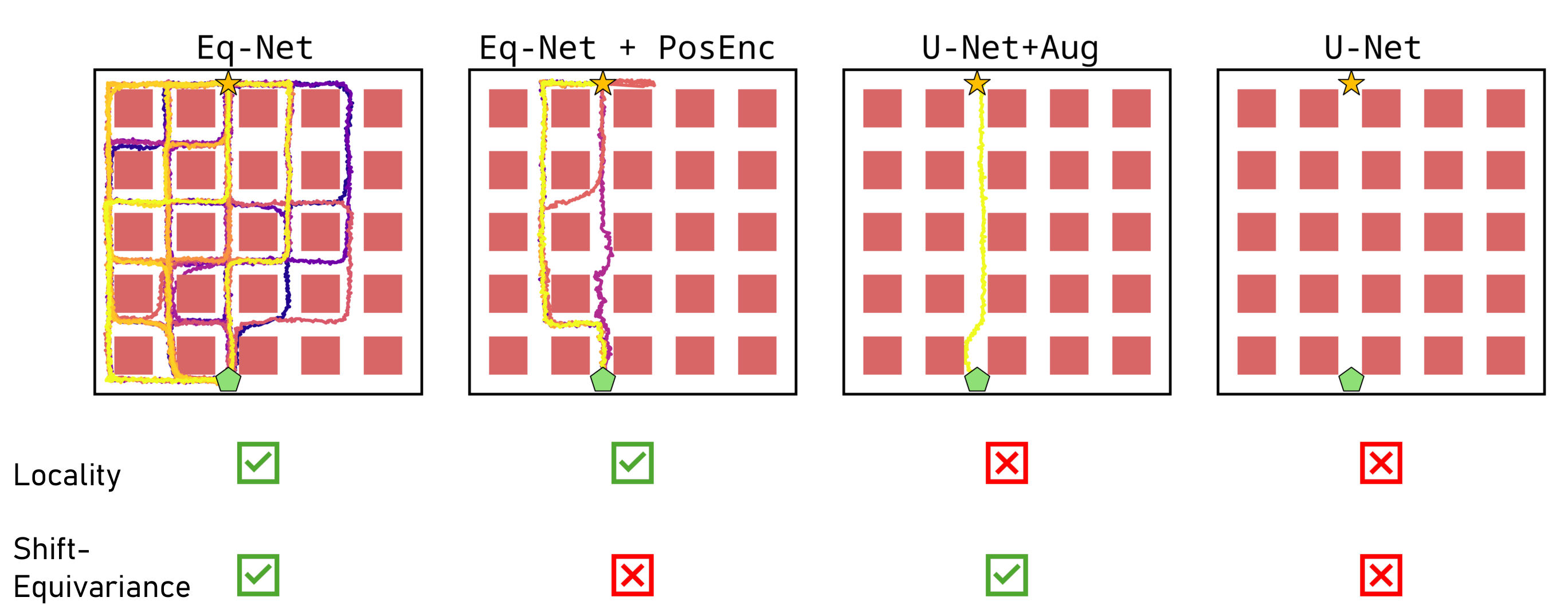
Locality matters more than equivariance
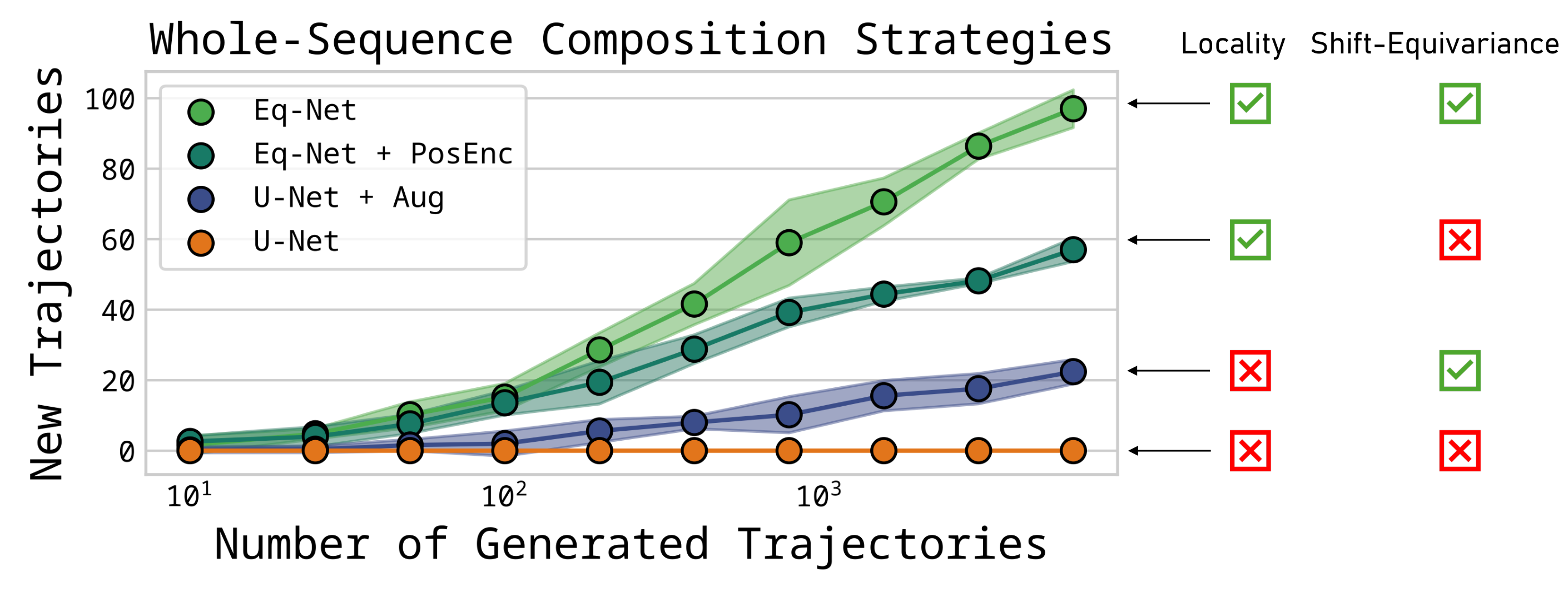
Positional encodings remove shift-equivariance from Eq-Net, and data augmentation adds it to U-Net. Locality alone helps more than shift-equivariance alone, and both together work best
Locality matters more than equivariance
Different routes to compositionality
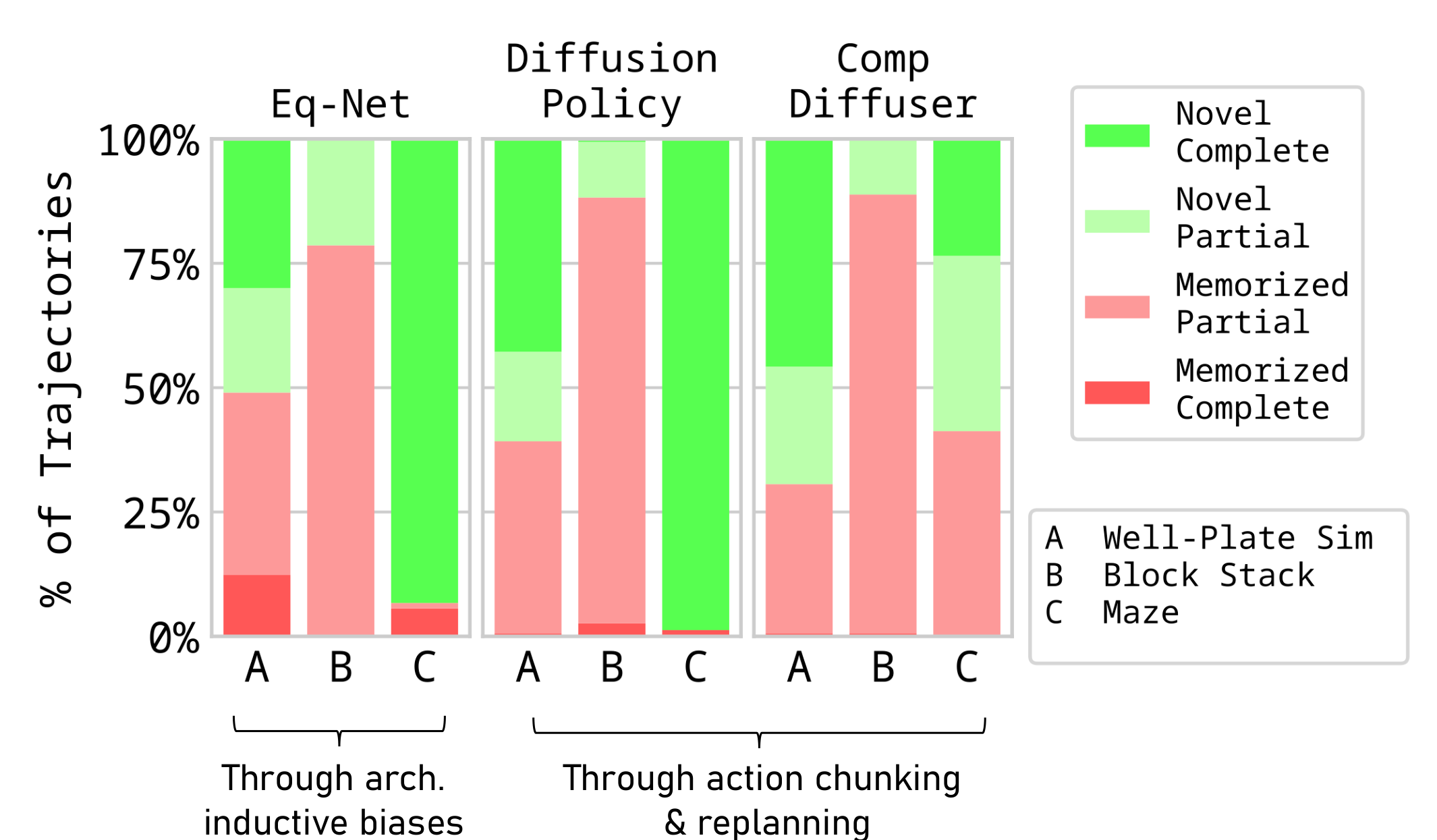
Eq-Net: through architectural inductive biases (locality and shift-equivariance)
Diffusion Policy and CompDiffuser: through action chunking and replanning