Week 2: Introduction to Optimal Control & Model-Based RL
Florian Shkurti
Today’s agenda
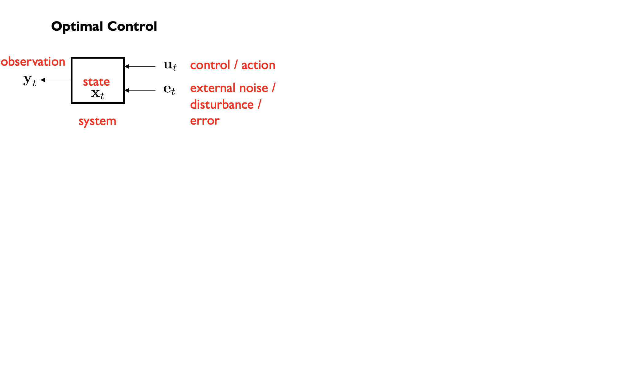
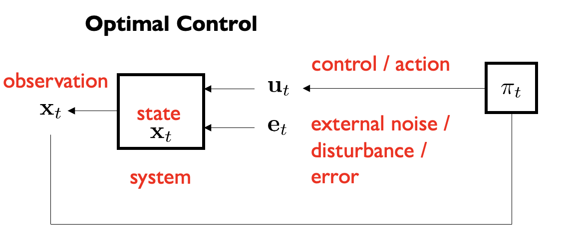
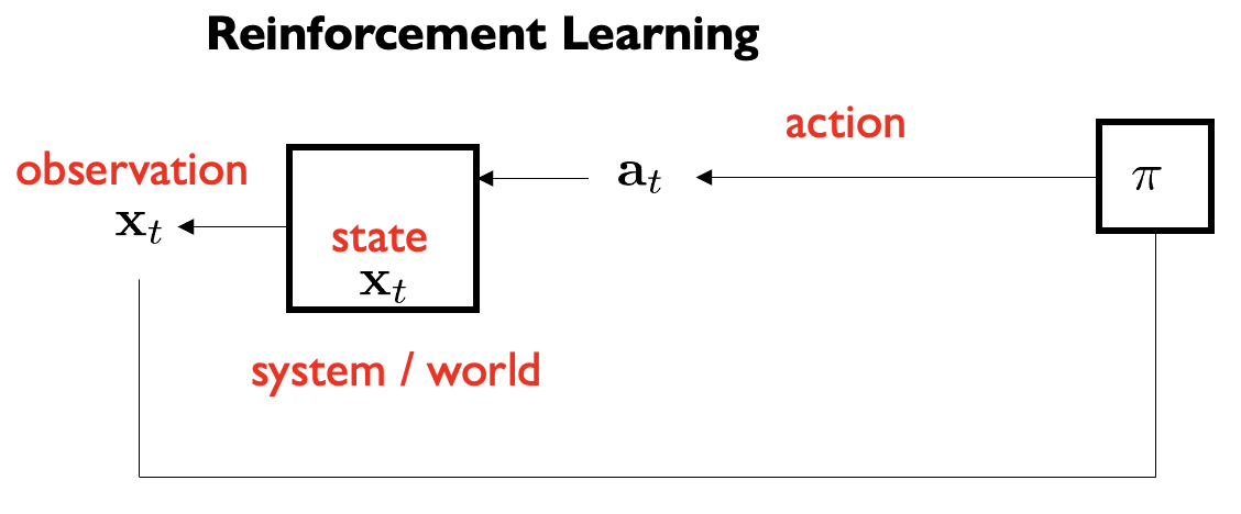
• Intro to Control & Reinforcement Learning
• Linear Quadratic Regulator (LQR)
• Iterative LQR
• Model Predictive Control
• Learning dynamics and model-based RL
• Model Predictive Path Integral Control (MPPI)
• Cross-Entropy Method (CEM)
\(\qquad \qquad \qquad \uparrow\)
Optimal state-action value function:
“if you land at state \(\mathbf{x}_t\), and you commit
to first execute action \(\mathbf{a}_t\), and then
follow the optimal actions/policy, how much
reward will you accumulate?”
Value function of policy \(\pi\): “if you land at state \(x_t\) and you follow policy \(\pi\) what is the expected reward you will accumulate?” \(\downarrow\)
State-action value function of policy \(\pi\):
“if you land at state \(\textbf{x}_t\), and you commit
to first execute action \(\textbf{a}_t\), and then follow
policy \(\pi\) how much reward will you
accumulate in expectation?” \(\downarrow\)
\[
\textcolor{red}{\swarrow \text{For finite time horizon} \searrow}
\]
State-action value
function of policy \(\pi\)\(\downarrow\)
Today’s agenda
• Intro to Control & Reinforcement Learning
• Linear Quadratic Regulator (LQR)
• Iterative LQR
• Model Predictive Control
• Learning dynamics and model-based RL
• Model Predictive Path Integral Control (MPPI)
• Cross-Entropy Method (CEM)
• You know the dynamics model of the system
• It is linear: \(\mathbf{x}_{t+1} = A\mathbf{x}_t + B\mathbf{u}_t\)
\(\qquad \qquad \qquad \qquad \uparrow\)
State at the next time step
\[
\mathbb{R}^d
\]
\[
A \in \mathbb{R}^{d \times d}
\]
\(\qquad \uparrow\)
Control / command / action applied to the system
\[
\mathbb{R}^k
\]
\[
B \in \mathbb{R}^{d \times k}
\]
Which systems are linear?
✓ • Omnidirectional robot
\[
\begin{align}
x_{t+1} &= x_t + v_x(t)\delta t \\
y_{t+1} &= y_t + v_y(t)\delta t \\
\theta_{t+1} &= \theta_t + \omega_z(t)\delta t
\end{align}
\quad \Rightarrow \quad
\]
\[
\mathbf{x}_{t+1} = I\mathbf{x}_t + \delta t I \mathbf{u}_t
\]\[
\begin{align}
A &= I \\
B &= \delta t I
\end{align}
\]
X • Simple Car
\[
\begin{align}
x_{t+1} &= x_t + v_x(t)\cos(\theta_t)\delta t \\
y_{t+1} &= y_t + v_x(t)\sin(\theta_t)\delta t \\
\theta_{t+1} &= \theta_t + \omega_z\delta t
\end{align}
\quad \Rightarrow \quad
\]
\[
\mathbf{x}_{t+1} = I\mathbf{x}_t + \begin{bmatrix}
\delta t\cos(\theta_t) & 0 & 0 \\
0 & \delta t\sin(\theta_t) & 0 \\
0 & 0 & \delta t
\end{bmatrix} \mathbf{u}_t
\]\[
\begin{align}
A &= I \\
B &= B(x_t) \\
\end{align}
\]
The goal of LQR
If we want to stabilize around \(x^*\) then let \(x\) – \(x^*\) be the state \(\downarrow\)
• Stabilize the system around state \(x_t = 0\) with control \(u_t = 0\)
• Then \(x_{t+1} = 0\) and the system will remain at zero forever
LQR: assumptions
• You know the dynamics model of the system
• It is linear: \(\mathbf{x}_{t+1} = Ax_t + Bu_t\)
• There is an instantaneous cost associated with being at state \(x_t\) and taking the action : \(\mathbf{u}_t: c(\mathbf{x}_t, \mathbf{u}_t) = \mathbf{x}_t^T Q \mathbf{x}_t + \mathbf{u}_t^T R \mathbf{u}_t\)
\(\color{red}\uparrow\) Quadratic state cost: Penalizes deviation from the zero vector
\(\color{red}\nwarrow\) Quadratic control cost: Penalizes high control signals
\(\color{red}\uparrow\)
\(\color{red}\nearrow\)
Square matrices Q and R must be positive definite: \(Q = Q^T\) and \(\forall x, x^T Q x > 0\) \(R = R^T\) and \(\forall u, u^T R u > 0\) i.e. positive cost for ANY nonzero state and control vector
Finite-Horizon LQR
• Idea: finding controls is an optimization problem
• Compute the control variables that minimize the cumulative cost
We could solve this as a constrained nonlinear optimization problem. But, there is a better way: we can find a closed-form solution.
Open-loop plan:
Given first state, compute action sequence
Finding the LQR controller in closed-form by recursion
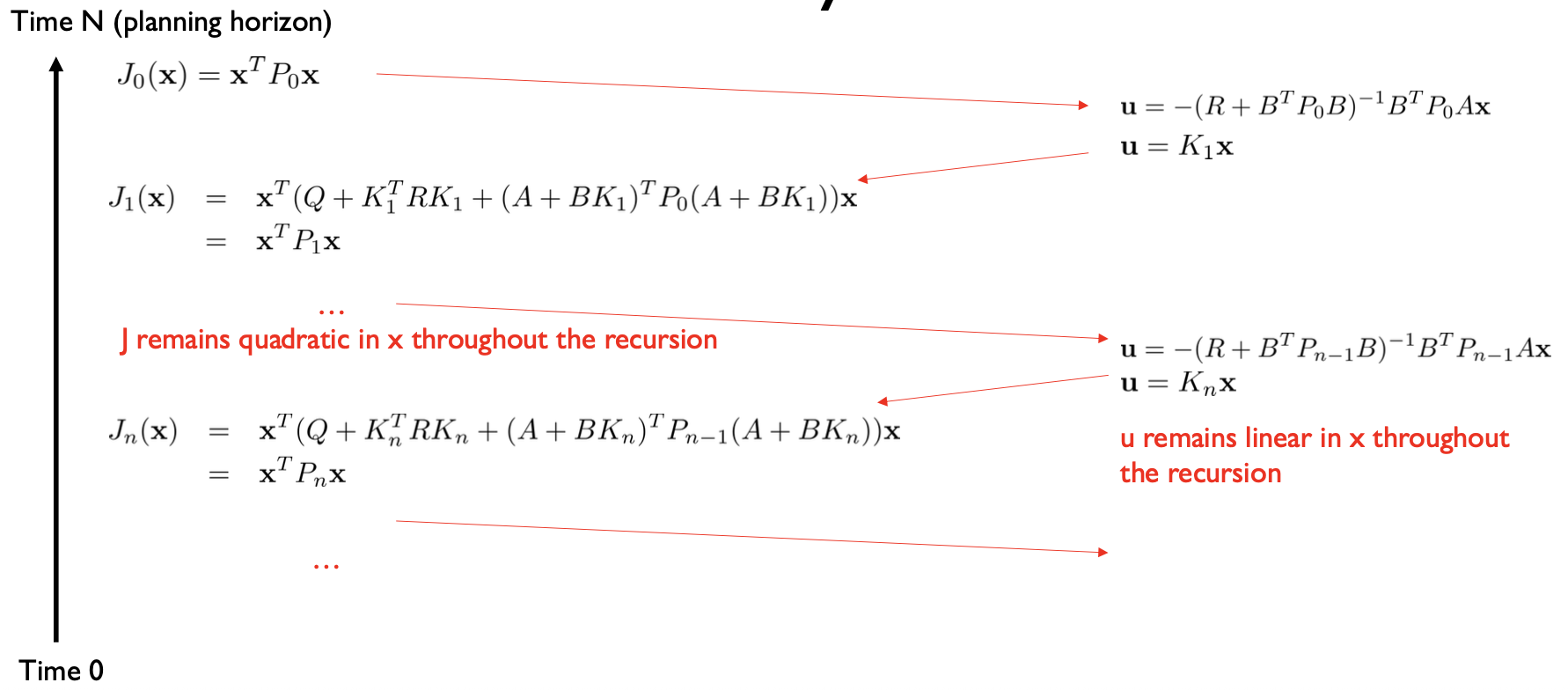
• Let \(J_n(x)\) denote the cumulative cost-to-go starting from state \(x\) and moving for \(n\) time steps.
• I.e. cumulative future cost from now till \(n\) more steps
• \(J_0(x) = x^TQx\) is the terminal cost of ending up at state \(x\), with no actions left to perform. Recall that \(c(x, u) = x^TQx + \cancel{u^T R u}\)
Q: What is the optimal cumulative cost-to-go function with 1 time step left?
Finding the LQR controller in closed-form by recursion
\(J_0(x) = x^TQx\)
For notational convenience later on, let’s define \(P_0 = Q\)
\[\begin{align}
J_1(\mathbf{x}) &= \min_{\mathbf{u}} \underbrace{[\mathbf{x}^T Q \mathbf{x} + \mathbf{u}^T R \mathbf{u} + J_0(A\mathbf{x} + B\mathbf{u})]}_{\color{red}\text{In RL this would be the state-action value function}} \\
\end{align}\]
Bellman Update
Dynamic Programming Value Iteration
Finding the LQR controller in closed-form by recursion
So, the optimal control for the last time step is: \(\mathbf{u} = -(R + B^T P_0 B)^{-1} B^T P_0 A \mathbf{x}\) \(\mathbf{u} = K_1 \mathbf{x}\)
Linear controller in terms of the state
We computed the location of the minimum. Now, plug it back in and compute the minimum value
Finding the LQR controller in closed-form by recursion
\[\begin{align}
J_0(\mathbf{x}) &= \mathbf{x}^TP_0\mathbf{x}\\
J_1(\mathbf{x}) &= \mathbf{x}^T Q \mathbf{x} + \mathbf{x}^T A^T P_0 A\mathbf{x} + \min_{\mathbf{u}} [\mathbf{u}^T R \mathbf{u} + 2\mathbf{u}^T B^T P_0 A\mathbf{x} + \mathbf{u}^T B^T P_0 B\mathbf{u}] \\
&= \mathbf{x}^T (\underbrace{Q + K_1^T R K_1 + (A + B K_1)^T P_0 (A + B K_1)}_{P_1}) \mathbf{x}
\end{align}\]
Q: Why is this a big deal?
A: The cost-to-go function remains quadratic after the first recursive step.
Finding the LQR controller in closed-form by recursion
Finite-Horizon LQR: algorithm summary
\(P_0 = Q\)
// n is the number of steps left
Potential problem for controls \(\mathbf{u}\) of dimension \(k\) >> 100:
Matrix inversion is expensive: \(O(k^{2.3})\) for the best known algorithm and \(O(k^3)\) for Gaussian Elimination. \(\swarrow\)
for n = 1…N
\(K_n = -(R + B^T P_{n-1} B)^{-1} B^T P_{n-1} A\) \(P_n = Q + K_n^T R K_n + (A + B K_n)^T P_{n-1} (A + B K_n)\)
One pass backward in time:
Matrix gains are precomputed based on the dynamics and the instantaneous cost
Optimal control parameters for time t = N – n are computed backwards in time: \(\mathbf{u}_t = K_t \mathbf{x}_t\) with cost-to-go \(J_t(\mathbf{x}) = \mathbf{x}^T P_t \mathbf{x}\), whereas the states are predicted forward in time according to linear dynamics
One pass forward in time: predict states, compute controls and cost-to-go
LQR: general form of dynamics and cost functions
Even though we assumed
we can also accommodate
\(\mathbf{x}_{t+1} = A \mathbf{x}_t + B \mathbf{u}_t\)
Then the form of the optimal policy is the same as in LQR \(\mathbf{u}_{t} = K_t \mathbf{x}_t + \mathbf{k}_t\)
No need to change the algorithm, as long as you observe the state at each step (closed-loop policy)
Linear Quadratic Gaussian LQG
LQR summary
Advantages:
If system is linear LQR gives the optimal controller that takes the system’s state to 0 (or the desired target state, same thing)
Drawbacks:
Linear dynamics
How can you include obstacles or constraints in the specification?
Not easy to put bounds on control values
Today’s agenda
• Intro to Control & Reinforcement Learning • Linear Quadratic Regulator (LQR)
• Iterative LQR
• Model Predictive Control
• Learning dynamics and model-based RL
• Model Predictive Path Integral Control (MPPI)
• Cross-Entropy Method (CEM)
Apply LQR backward pass on the approximate dynamics \(\tilde{f}(\delta \mathbf{x}_t, \delta \mathbf{u}_t)\) and cost \(\tilde{c}(\delta \mathbf{x}_t, \delta \mathbf{u}_t)\) to compute controller and cost-to-go parameters.
Do an LQR forward pass to get \(\delta \mathbf{u}_t\) and \(\delta \mathbf{x}_t\) and update state and action sequence and \(\bar{x}_0, \ldots, \bar{x}_N\) and \(\bar{u}_0, \ldots, \bar{u}_N\)
Iterative LQR: convergence & tricks
New state and action sequence in iLQR is not guaranteed to be close to the linearization point (so linear approximation might be bad)
Trick: try to penalize magnitude of \(\delta u_t\) and \(\delta x_t\)
Replace old LQR linearized cost with \((1 - \alpha) \, \tilde{c}(\delta \mathbf{x}_t, \delta \mathbf{u}_t) + \alpha \left( \| \delta \mathbf{x}_t \|^2 + \| \delta \mathbf{u}_t \|^2 \right)\)
Problem: Can get stuck in local optima, need to initialize well
Problem: Hessian might not be positive definite
Today’s agenda
• Intro to Control & Reinforcement Learning • Linear Quadratic Regulator (LQR) • Iterative LQR
• Model Predictive Control
• Learning dynamics and model-based RL
• Model Predictive Path Integral Control (MPPI)
• Cross-Entropy Method (CEM)
Open loop vs. closed loop
• The instances of LQR and iLQR that we saw were open-loop
• Commands are executed in sequence, without feedback
• Idea: what if we throw away all commands except the first
• We can execute the first command, and then replan Takes into account the changing state
Model Predictive Control
while True:
observe the current state \(x_0\)
run LQR/iLQR or LQG/iLQG or other planner to get \({u}_0, \ldots, {u}_{N-1}\)
Execute \(u_0\)
Possible speedups:
Don’t plan too far ahead with LQR
Execute more than one planned action
Warm starts and initialization
Use faster / custom optimizer (e.g. CPLEX, sequential quadratic programming)
• Intro to Control & Reinforcement Learning • Linear Quadratic Regulator (LQR) • Iterative LQR • Model Predictive Control
• Learning dynamics and model-based RL
• Model Predictive Path Integral Control (MPPI)
• Cross-Entropy Method (CEM)
Learning a dynamics model
Idea #1: Collect dataset \(D = \{(x_t, u_t, x_{t+1})\}\)
do supervised learning to minimize \(\sum_{t} \left\| f_{\theta}(x_t, u_t) - x_{t+1} \right\|^2\)
and then use the learned model for planning
Possibly a better idea: instead of minimizing single-step prediction errors, minimize multi-step errors.
See “Improving Multi-step Prediction of Learned Time Series Models” by Venkatraman, Hebert, Bagnell
Possibly a better idea: instead of predicting next state predict next change in state.
See “PILCO: A Model-Based and Data-Efficient Approach to Policy Search” by Deisenroth, Rasmussen
Plan through \(f_{\theta}(x_t, u_t)\) to get actions
Execute first action, observe new state \(x_{t+1}\)
Append \((x_t, u_t, x_{t+1})\) to \(D\)
How do we plan through a learned model?
iLQR needs \(\frac{\partial f}{\partial x}, \frac{\partial f}{\partial u}\) and \(\nabla^2 c\): the model and the cost must be smooth, and the Hessian should be positive definite
Often that is not the case:
\(f_\theta\) is a neural network (gradients exist but are noisy, and the linearization can be very poor far from the data)
\(f\) is a black-box simulator with contacts (no gradients at all)
\(c\) is discontinuous, e.g. an indicator for collisions or reaching a goal region
Idea: don’t differentiate at all. Sample many action sequences, roll them out through the model in parallel, and average the good ones
Model Predictive Path Integral Control (MPPI)
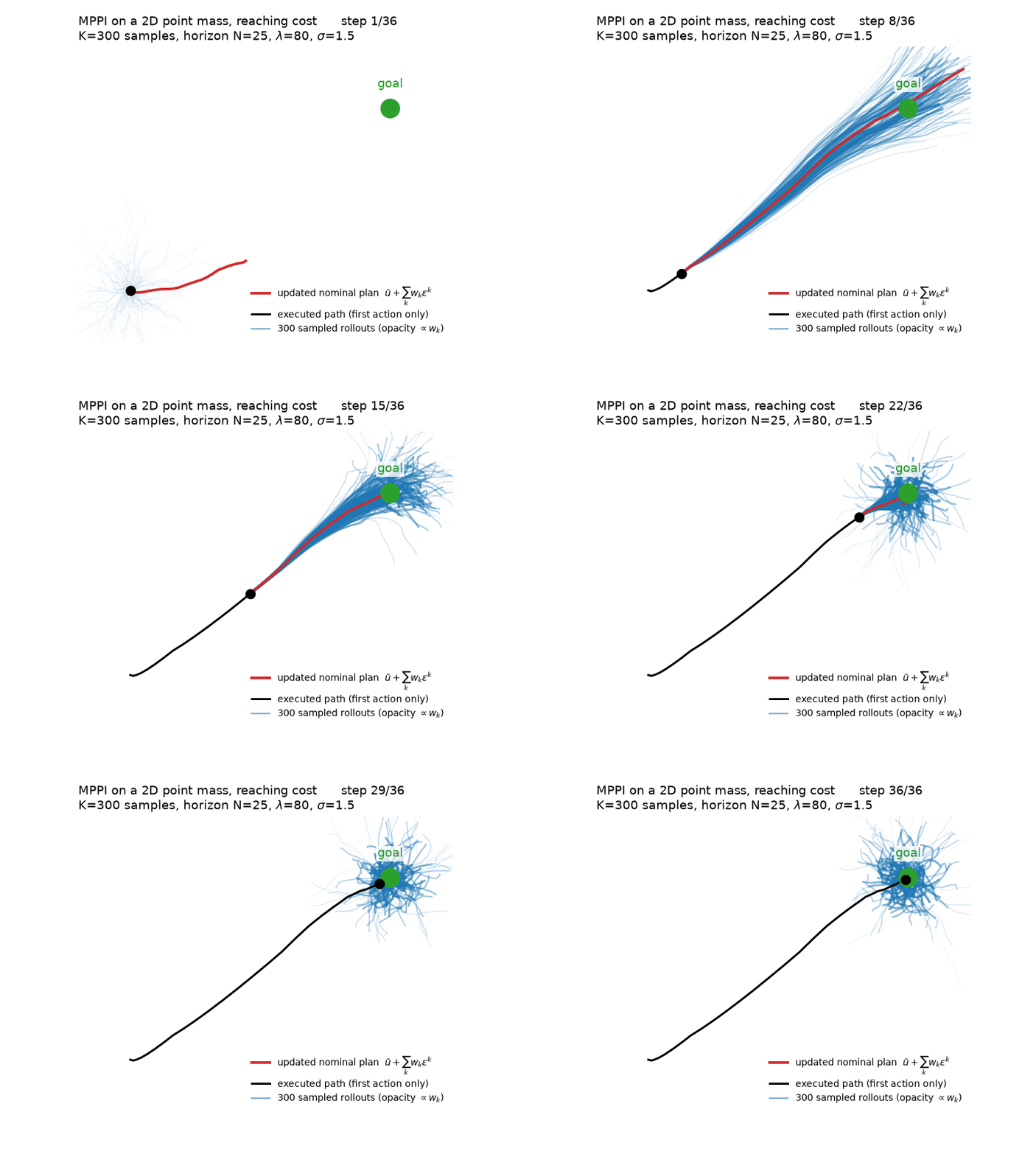
Given the current state \(x_0\) and a nominal action sequence \(\bar{u}_0, \ldots, \bar{u}_{N-1}\) (e.g. last plan, shifted by one step):
• Blue: the \(K\) sampled rollouts, opacity \(\propto w_k\)
• Red: the new nominal plan \(\bar{u} + \sum_k w_k \epsilon^k\)
• Black: the executed path (only \(\bar{u}_0\) is applied, then replan)
Notice how the samples are spread out when far from the goal and collapse around it once we arrive: the weights and the warm start do the work, no gradients needed
MPPI: properties & tricks
\(\lambda \to 0\): only keep the best rollout (greedy). \(\lambda \to \infty\): plain average of all samples. In between: a smoothed, weighted average of the good samples
Derivative-free: works with any model you can evaluate, including neural networks and simulators with contact, and with discontinuous costs
Warm start is essential: reuse last plan shifted by one step. With a good warm start, one MPPI update per control step is often enough
Problems: \(K\) needs to grow with the action dimension and horizon; exploration noise \(\Sigma\) has to be tuned; no local convergence guarantee like iLQR
See “Model Predictive Path Integral Control: From Theory to Parallel Computation”
“Information Theoretic MPC for Model-Based Reinforcement Learning” by Williams, Aldrich, Theodorou et al. (2017),
where MPPI is used to drive the AutoRally car aggressively with a learned neural network dynamics model
A closely related idea: the Cross-Entropy Method (CEM)
• MPPI keeps a single nominal sequence \(\bar{u}\) and nudges it with a weighted average of the noise
• CEM instead maintains a distribution over action sequences, \(q(u_{0:N-1}) = \mathcal{N}(\mu, \Sigma)\), and iteratively refits it to the best samples
• Comes from rare-event simulation (Rubinstein, 1997): to estimate the probability of a rare event, iteratively move the sampling distribution towards the region where the event happens
For optimization the “rare event” is “cost below the current threshold”, and the distribution concentrates on low-cost action sequences
Cross-Entropy Method (CEM) for planning
Given the current state \(x_0\) and an initial distribution \(\mu_t, \Sigma_t\) over actions (e.g. \(\mu\) = last plan shifted by one step, \(\Sigma\) reset to a large value):
Roll out each one through the model: \(x^k_{t+1} = f(x^k_t, u^k_t)\), starting from \(x_0\)
Compute the cost of each rollout: \(S_k = \sum_{t=0}^{N-1} c(x^k_t, u^k_t) + c_N(x^k_N)\)
Keep the \(M \ll K\) lowest-cost sequences, the elites\(\mathcal{E}\)
Refit the distribution to the elites: \[
\mu_t \leftarrow \frac{1}{M} \sum_{k \in \mathcal{E}} u^k_t \qquad \Sigma_t \leftarrow \frac{1}{M} \sum_{k \in \mathcal{E}} (u^k_t - \mu_t)(u^k_t - \mu_t)^T
\]
Execute \(\mu_0\), observe the new state, shift \(\mu\), repeat (MPC)
Step 5 is a maximum-likelihood fit of a Gaussian to the elites, i.e. it minimizes the cross-entropy between the elite distribution and \(q\), hence the name
CEM in action: reaching a goal
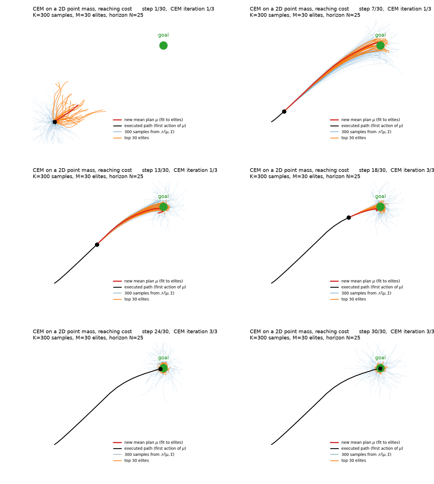
Same point mass and reaching cost as in the MPPI example
Each frame is one CEM iteration; 3 iterations per control step
• Blue: the \(K\) samples from \(\mathcal{N}(\mu, \Sigma)\)
• Orange: the \(M\) elites
• Red: the new mean plan \(\mu\), fit to the elites
• Black: the executed path (only \(\mu_0\) is applied, then replan)
Watch the sample cloud shrink within each control step as \(\Sigma\) is refit to the elites, then widen again when \(\Sigma\) is reset for the next step
CEM vs. MPPI
CEM
MPPI
What is updated
mean \(\mu\)and covariance \(\Sigma\)
nominal sequence \(\bar{u}\) only (\(\Sigma\) fixed)
How samples are used
hard threshold: top \(M\) elites, equal weight
soft weights \(w_k \propto \exp(-S_k / \lambda)\) on all samples
Iterations per step
usually several (distribution needs to shrink)
often one, thanks to warm start
Hyperparameters
\(K\), \(M\), initial \(\Sigma\), # iterations
\(K\), \(\lambda\), \(\Sigma\)
Behavior
more exploitative, converges quickly, can collapse too early
smoother updates, more robust to noisy costs
Both are derivative-free, embarrassingly parallel, and work with learned models and discontinuous costs
Both scale poorly with action dimension and horizon: a Gaussian over \(N \cdot \dim(u)\) variables gets very wide, very fast
Tricks: keep the top elites across iterations, smooth \(\mu\) over time (colored noise), sample in a low-dimensional space of action splines
CEM was the planner of choice in many model-based RL papers, e.g. “Deep RL in a Handful of Trials using Probabilistic Dynamics Models” (PETS, Chua et al. 2018) and “Learning Latent Dynamics for Planning from Pixels” (PlaNet, Hafner et al. 2019)
Today’s agenda
• Intro to Control & Reinforcement Learning • Linear Quadratic Regulator (LQR) • Iterative LQR • Model Predictive Control • Learning dynamics and model-based RL • Model Predictive Path Integral Control (MPPI) • Cross-Entropy Method (CEM)
• Appendix
Appendix #1 (optional reading) LQR extensions: time-varying systems
• What can we do when \(x_{t+1} = A_t x_t + B_t u_t\) and \(c(x_t, u_t) = x_t^T Q x_t + u_t^T R u_t\) ?
• Turns out, the proof and the algorithm are almost the same
Optimal controller for n-step horizon is \(u_n = K_n x_n\) with cost-to-go \(J_n(x) = x^T P_n x\)
Appendix #2 (optional reading) Why not use PID control?
• We could, but:
• The gains for PID are good for a small region of state-space.
• System reaches a state outside this set → becomes unstable
• PID has no formal guarantees on the size of the set
• We would need to tune PID gains for every control variable.
• If the state vector has multiple dimensions it becomes harder to tune every control variable in isolation. Need to consider interactions and correlations.
• We would need to tune PID gains for different regions of the state-space and guarantee smooth gain transitions
• This is called gain scheduling, and it takes a lot of effort and time
LQR addresses these problems
Appendix #3 (optional reading) Examples of models and solutions with LQR
LQR example #1: omnidirectional vehicle with friction
• Similar to double integrator dynamical system, but with friction:
\[
\underset{\color{red}\text{Force applied to the vehicle}}{\underline{m\ddot{p}}} = \underset{\color{red}\text{Control applied to the vehicle}}{\underline{\mathbf{u}}} - \underset{\color{red}\text{Friction opposed to motion}}{\underline{\alpha \dot{p}}}
\]
LQR example #1: omnidirectional vehicle with friction
• Similar to double integrator dynamical system, but with friction:
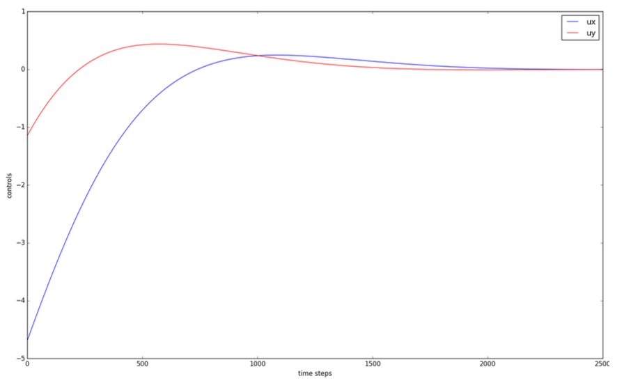
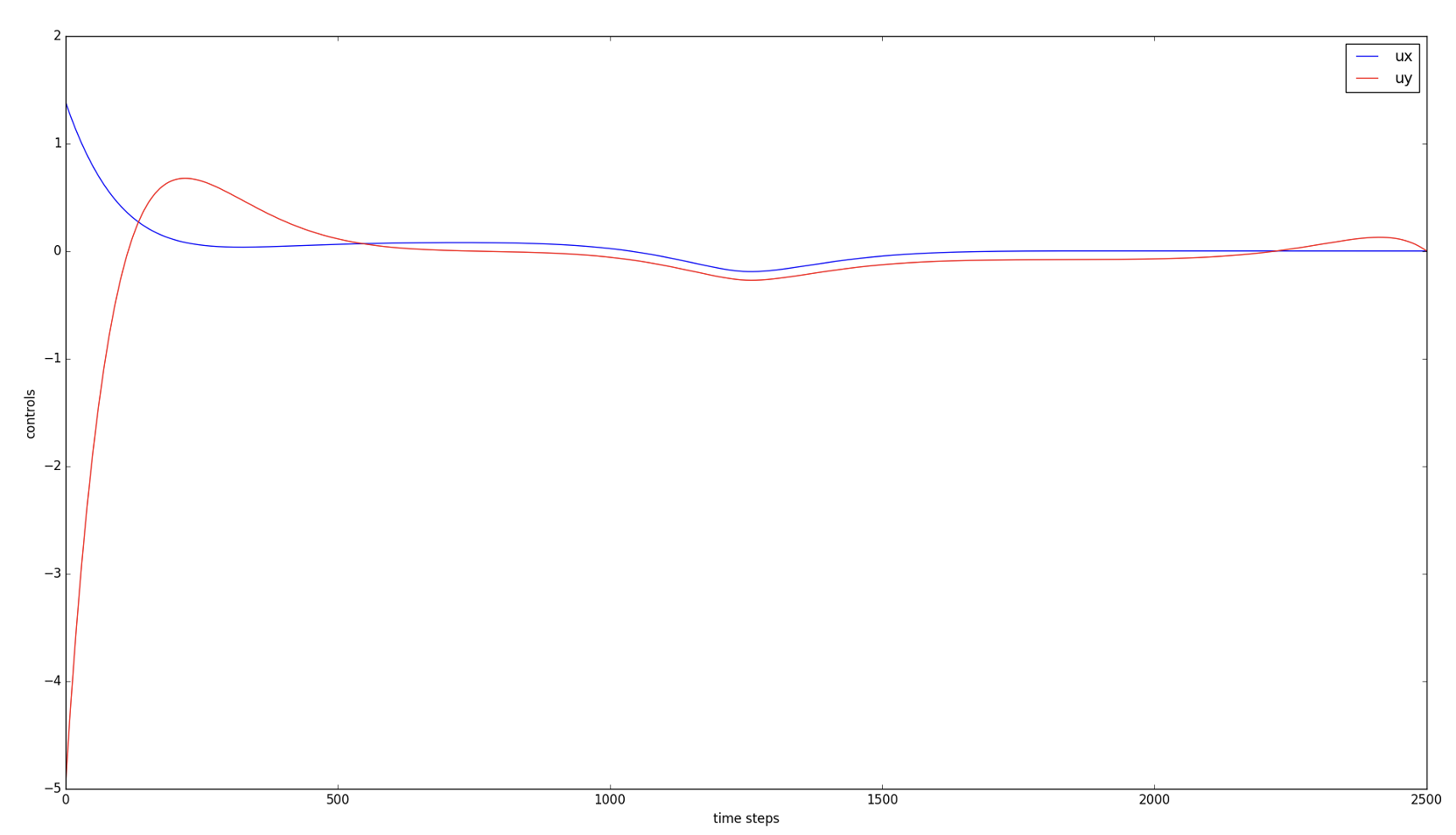
Notice how the controls tend to zero.
It’s because the state tends to zero as well.
Also note that in the current LQR framework,
we have not included hard constraints on the controls,
i.e. upper or lower bounds. We only penalize large norm for controls.
LQR example #1: omnidirectional vehicle with friction
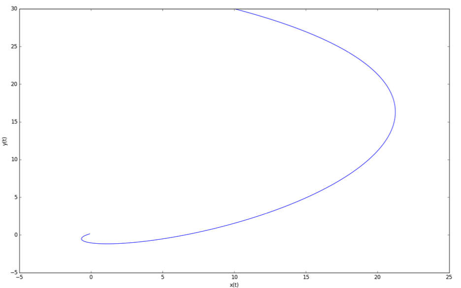
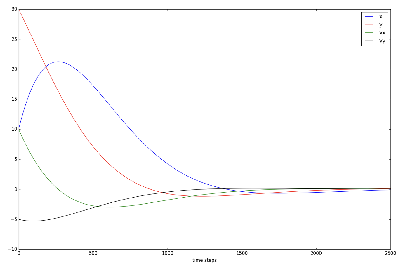
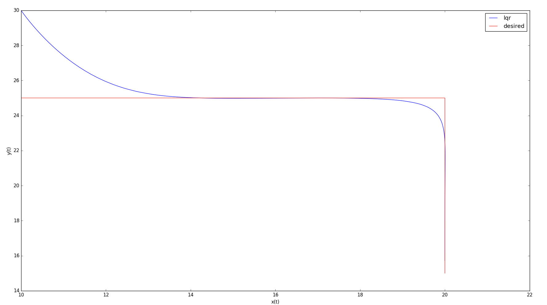
With initial state \(\mathbf{x}_0 = \begin{bmatrix}10 \\ 30\\ 10\\ -5\end{bmatrix}\)